87  Raster and vector

Keywords

raster, vector, experimental plots, clip

Vector and raster layers are fundamental data formats in Geographic Information Systems (GIS). Vector data represents geographic features as points, lines, and polygons. Vector data is used for precise representation of features like roads or county boundaries. Raster data represents the Earth’s surface as a grid of cells, where each cell stores a single value or attribute. Raster data is often used for continuous phenomena such as elevation or land cover.

In this tutorial we will vegetation patterns across multiple watersheds of the Konza Prairie Biological Station near Manhattan, KS.

# Import modules
import numpy as np
import geopandas as gpd
import xarray as xr
import matplotlib.pyplot as plt
from matplotlib import colors

Read vector layer

# Read file with watersheds
vector_path = '../datasets/spatial/konza_watersheds.geojson'
gdf = gpd.read_file(vector_path)
gdf.head(3)

	CODE_1	NAME_1	AREA	PERIMETER	ACRES	HECTARES_1	DATAID_1	DATACODE_2	geometry
0	0R1A	R1A	484815.196184	2939.146533	119.800444	48.481520	GIS0321	GIS032	POLYGON ((707045.277 4327611.469, 707038.577 4...
1	R20A	R20A	263364.016292	2509.563160	65.078666	26.336402	GIS0322	GIS032	POLYGON ((707080.980 4327453.175, 707080.987 4...
2	002A	2A	283017.160279	2417.724921	69.935063	28.301716	GIS0323	GIS032	POLYGON ((707362.870 4327681.792, 707364.460 4...

# Visualize vector map of watersheds
gdf.plot(facecolor='None', edgecolor='k')
plt.title('Konza Watersheds')
plt.xlabel('Easting (meters)')
plt.ylabel('Northin (meters)')
plt.show()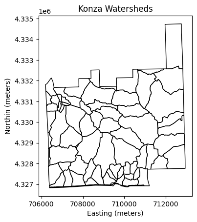

# Display coordiante reference system of vector layer
print(gdf.crs)

EPSG:26914

The first step to perform spatial operations between vector and raster layers is to have both data sources in the same coordinate reference system. Our vector layer has geometries in projected coordinates (meters), but the raster datasets will be in geographic coordinates.

To perform operations that involve distance computations is best to have both datasets in projected coordiantes. To perform other operations like clipping layers, then both geographic and projected coordinates should perform similarly. In this example we will convert the vector layer to geographic coordinates.

# Change coordinate reference system from projected to geographic
gdf.to_crs(epsg=4326, inplace=True)
gdf.head(3)

	CODE_1	NAME_1	AREA	PERIMETER	ACRES	HECTARES_1	DATAID_1	DATACODE_2	geometry
0	0R1A	R1A	484815.196184	2939.146533	119.800444	48.481520	GIS0321	GIS032	POLYGON ((-96.60663 39.07307, -96.60671 39.073...
1	R20A	R20A	263364.016292	2509.563160	65.078666	26.336402	GIS0322	GIS032	POLYGON ((-96.60627 39.07163, -96.60627 39.071...
2	002A	2A	283017.160279	2417.724921	69.935063	28.301716	GIS0323	GIS032	POLYGON ((-96.60294 39.07362, -96.60292 39.073...

Note

If the cell above still shows the geometry column in projected coordinates, consider forcing the dataset to the correct coordinate reference system when reading the file, like this:

`gdf = gpd.read_file(vector_path).set_crs(‘epsg:26914’, allow_override=True)

# Visualize vector map of watersheds
gdf.plot(facecolor='None', edgecolor='k')
plt.title('Konza Watersheds')
plt.xlabel('Longitude')
plt.ylabel('Latitude')
plt.show()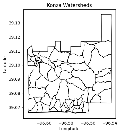

Read raster layer

The raster layer is a multi-band geo-referenced image at 10-meter spatial resolution obtained from Sentinel-2 satellite. Image data type is unsigned 16-bit (2^{16}). The bands are as follows:

• Band 1: Senteninel B03 (green, 560 nm)
• Band 2: Sentinel B04 (red, 665 nm)
• Band 3: Sentinel B08 (near infrared, 842 nm)

The image was downloaded using Sentinel Hub: https://www.sentinel-hub.com/explore/eobrowser/

# Load raster layer
raster_path = '../datasets/spatial/2024-04-03_Sentinel-2_L2A_B03_B04_B08-16bit.tiff'
raster = xr.open_dataarray(raster_path)
raster

<xarray.DataArray 'band_data' (band: 3, y: 1060, x: 1461)>
[4645980 values with dtype=float32]
Coordinates:
  * band         (band) int64 1 2 3
  * x            (x) float64 -96.66 -96.66 -96.66 ... -96.53 -96.53 -96.53
  * y            (y) float64 39.15 39.15 39.15 39.15 ... 39.06 39.06 39.06 39.06
    spatial_ref  int64 ...
Attributes:
    AREA_OR_POINT:           Area
    TIFFTAG_RESOLUTIONUNIT:  1 (unitless)
    TIFFTAG_XRESOLUTION:     1
    TIFFTAG_YRESOLUTION:     1

xarray.DataArray

'band_data'

• band: 3
• y: 1060
• x: 1461

• ...

  [4645980 values with dtype=float32]

• Coordinates: (4)
  • band
    (band)
    int64
    1 2 3

    array([1, 2, 3])

  • x
    (x)
    float64
    -96.66 -96.66 ... -96.53 -96.53

    array([-96.664536, -96.664446, -96.664356, ..., -96.533314, -96.533224,
           -96.533134])

  • y
    (y)
    float64
    39.15 39.15 39.15 ... 39.06 39.06

    array([39.154246, 39.154156, 39.154066, ..., 39.059142, 39.059052, 39.058962])

  • spatial_ref
    ()
    int64
    ...

    crs_wkt :

    GEOGCS["WGS 84",DATUM["WGS_1984",SPHEROID["WGS 84",6378137,298.257223563,AUTHORITY["EPSG","7030"]],AUTHORITY["EPSG","6326"]],PRIMEM["Greenwich",0,AUTHORITY["EPSG","8901"]],UNIT["degree",0.0174532925199433,AUTHORITY["EPSG","9122"]],AXIS["Latitude",NORTH],AXIS["Longitude",EAST],AUTHORITY["EPSG","4326"]]

    semi_major_axis :

    6378137.0

    semi_minor_axis :

    6356752.314245179

    inverse_flattening :

    298.257223563

    reference_ellipsoid_name :

    WGS 84

    longitude_of_prime_meridian :

    0.0

    prime_meridian_name :

    Greenwich

    geographic_crs_name :

    WGS 84

    horizontal_datum_name :

    World Geodetic System 1984

    grid_mapping_name :

    latitude_longitude

    spatial_ref :

    GEOGCS["WGS 84",DATUM["WGS_1984",SPHEROID["WGS 84",6378137,298.257223563,AUTHORITY["EPSG","7030"]],AUTHORITY["EPSG","6326"]],PRIMEM["Greenwich",0,AUTHORITY["EPSG","8901"]],UNIT["degree",0.0174532925199433,AUTHORITY["EPSG","9122"]],AXIS["Latitude",NORTH],AXIS["Longitude",EAST],AUTHORITY["EPSG","4326"]]

    GeoTransform :

    -96.664581 9.000136892538973e-05 0.0 39.154291 0.0 -8.997547169811285e-05

    [1 values with dtype=int64]

• Indexes: (3)
  • band
    PandasIndex

    PandasIndex(Int64Index([1, 2, 3], dtype='int64', name='band'))

  • x
    PandasIndex

    PandasIndex(Float64Index([-96.66453599931553,  -96.6644459979466, -96.66435599657768,
                  -96.66426599520875, -96.66417599383983,  -96.6640859924709,
                  -96.66399599110198, -96.66390598973305, -96.66381598836414,
                   -96.6637259869952,
                  ...
                   -96.5339440130048, -96.53385401163587, -96.53376401026694,
                  -96.53367400889802, -96.53358400752909, -96.53349400616017,
                  -96.53340400479124, -96.53331400342232, -96.53322400205339,
                  -96.53313400068447],
                 dtype='float64', name='x', length=1461))

  • y
    PandasIndex

    PandasIndex(Float64Index([ 39.15424601226415,  39.15415603679246, 39.154066061320755,
                   39.15397608584906,  39.15388611037736,  39.15379613490566,
                  39.153706159433966, 39.153616183962264,  39.15352620849057,
                   39.15343623301887,
                  ...
                  39.059771766981136,  39.05968179150943,  39.05959181603774,
                   39.05950184056604,  39.05941186509434, 39.059321889622645,
                   39.05923191415095,  39.05914193867925,  39.05905196320755,
                   39.05896198773585],
                 dtype='float64', name='y', length=1060))

• Attributes: (4)

  AREA_OR_POINT :

  Area

  TIFFTAG_RESOLUTIONUNIT :

  1 (unitless)

  TIFFTAG_XRESOLUTION :

  1

  TIFFTAG_YRESOLUTION :

  1

# Display CRS for raster layer
print(raster.rio.crs)

EPSG:4326

# Create separate variables to easily keep track of each band
red = raster[1] # Red band
nir = raster[2] # NIR band

# Visualize raster files (1 band each)
plt.figure(figsize=(12,4))

plt.subplot(1,2,1)
plt.title('Red band')
red.plot(cmap='Spectral')

plt.subplot(1,2,2)
plt.title('NIR band')
nir.plot(cmap='Spectral')

plt.show()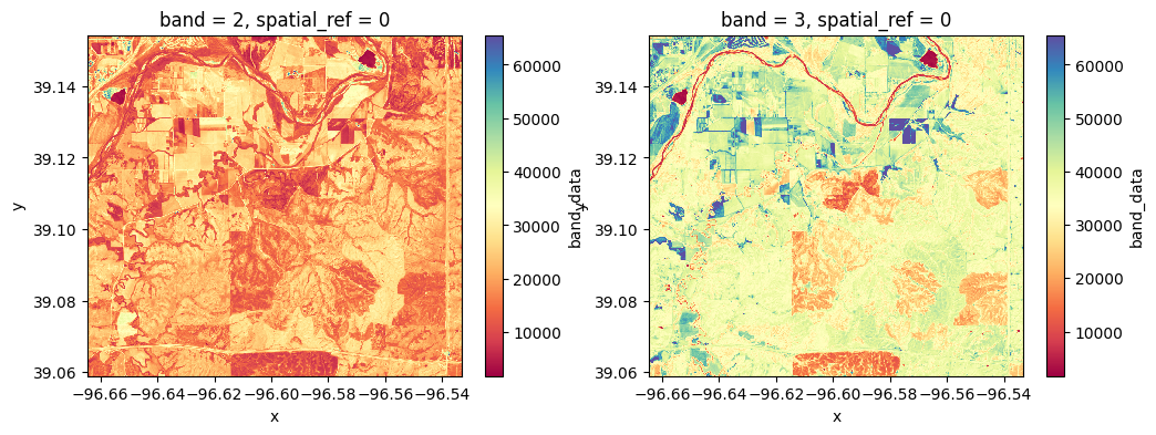

Compute NDVI

Normalized Difference Vegetation Index (NDVI) is a measure typically used in remote sensing to quantify and assess vegetation health and density. It is calculated using near-infrared (NIR) and red light reflectance values over an area as follows:

NDVI = \frac{NIR-Red}{NIR+Red}

NDVI values range from -1 to 1, where higher values indicate healthier and denser vegetation, typically falling between 0.2 and 0.8 for vegetation. Bare soil and rocks fall have values ranging from 0 to 0.2. Bodies of water like ponds, likes, rivers, and oceans typically have negative values close to -1.

# Calculate NDVI
ndvi = (nir - red)/(nir + red)
ndvi

<xarray.DataArray 'band_data' (y: 1060, x: 1461)>
array([[0.20274895, 0.20937616, 0.20950142, ..., 0.67129827, 0.66197807,
        0.6533825 ],
       [0.20902824, 0.21146326, 0.20774542, ..., 0.6241462 , 0.6243218 ,
        0.61213624],
       [0.2056777 , 0.20352827, 0.20263384, ..., 0.4648589 , 0.46888125,
        0.43359682],
       ...,
       [0.24272305, 0.24409018, 0.29347083, ..., 0.24446614, 0.245708  ,
        0.23017304],
       [0.23893936, 0.25726736, 0.30064335, ..., 0.23905072, 0.21922347,
        0.21036135],
       [0.25735095, 0.27477464, 0.32591128, ..., 0.21947752, 0.22523181,
        0.21821591]], dtype=float32)
Coordinates:
  * x            (x) float64 -96.66 -96.66 -96.66 ... -96.53 -96.53 -96.53
  * y            (y) float64 39.15 39.15 39.15 39.15 ... 39.06 39.06 39.06 39.06
    spatial_ref  int64 0

xarray.DataArray

'band_data'

• y: 1060
• x: 1461

• 0.2027 0.2094 0.2095 0.2019 0.2027 ... 0.2146 0.2195 0.2252 0.2182

  array([[0.20274895, 0.20937616, 0.20950142, ..., 0.67129827, 0.66197807,
          0.6533825 ],
         [0.20902824, 0.21146326, 0.20774542, ..., 0.6241462 , 0.6243218 ,
          0.61213624],
         [0.2056777 , 0.20352827, 0.20263384, ..., 0.4648589 , 0.46888125,
          0.43359682],
         ...,
         [0.24272305, 0.24409018, 0.29347083, ..., 0.24446614, 0.245708  ,
          0.23017304],
         [0.23893936, 0.25726736, 0.30064335, ..., 0.23905072, 0.21922347,
          0.21036135],
         [0.25735095, 0.27477464, 0.32591128, ..., 0.21947752, 0.22523181,
          0.21821591]], dtype=float32)

• Coordinates: (3)
  • x
    (x)
    float64
    -96.66 -96.66 ... -96.53 -96.53

    array([-96.664536, -96.664446, -96.664356, ..., -96.533314, -96.533224,
           -96.533134])

  • y
    (y)
    float64
    39.15 39.15 39.15 ... 39.06 39.06

    array([39.154246, 39.154156, 39.154066, ..., 39.059142, 39.059052, 39.058962])

  • spatial_ref
    ()
    int64
    0

    crs_wkt :

    GEOGCS["WGS 84",DATUM["WGS_1984",SPHEROID["WGS 84",6378137,298.257223563,AUTHORITY["EPSG","7030"]],AUTHORITY["EPSG","6326"]],PRIMEM["Greenwich",0,AUTHORITY["EPSG","8901"]],UNIT["degree",0.0174532925199433,AUTHORITY["EPSG","9122"]],AXIS["Latitude",NORTH],AXIS["Longitude",EAST],AUTHORITY["EPSG","4326"]]

    semi_major_axis :

    6378137.0

    semi_minor_axis :

    6356752.314245179

    inverse_flattening :

    298.257223563

    reference_ellipsoid_name :

    WGS 84

    longitude_of_prime_meridian :

    0.0

    prime_meridian_name :

    Greenwich

    geographic_crs_name :

    WGS 84

    horizontal_datum_name :

    World Geodetic System 1984

    grid_mapping_name :

    latitude_longitude

    spatial_ref :

    GEOGCS["WGS 84",DATUM["WGS_1984",SPHEROID["WGS 84",6378137,298.257223563,AUTHORITY["EPSG","7030"]],AUTHORITY["EPSG","6326"]],PRIMEM["Greenwich",0,AUTHORITY["EPSG","8901"]],UNIT["degree",0.0174532925199433,AUTHORITY["EPSG","9122"]],AXIS["Latitude",NORTH],AXIS["Longitude",EAST],AUTHORITY["EPSG","4326"]]

    GeoTransform :

    -96.664581 9.000136892538973e-05 0.0 39.154291 0.0 -8.997547169811285e-05

    array(0)

• Indexes: (2)
  • x
    PandasIndex

    PandasIndex(Float64Index([-96.66453599931553,  -96.6644459979466, -96.66435599657768,
                  -96.66426599520875, -96.66417599383983,  -96.6640859924709,
                  -96.66399599110198, -96.66390598973305, -96.66381598836414,
                   -96.6637259869952,
                  ...
                   -96.5339440130048, -96.53385401163587, -96.53376401026694,
                  -96.53367400889802, -96.53358400752909, -96.53349400616017,
                  -96.53340400479124, -96.53331400342232, -96.53322400205339,
                  -96.53313400068447],
                 dtype='float64', name='x', length=1461))

  • y
    PandasIndex

    PandasIndex(Float64Index([ 39.15424601226415,  39.15415603679246, 39.154066061320755,
                   39.15397608584906,  39.15388611037736,  39.15379613490566,
                  39.153706159433966, 39.153616183962264,  39.15352620849057,
                   39.15343623301887,
                  ...
                  39.059771766981136,  39.05968179150943,  39.05959181603774,
                   39.05950184056604,  39.05941186509434, 39.059321889622645,
                   39.05923191415095,  39.05914193867925,  39.05905196320755,
                   39.05896198773585],
                 dtype='float64', name='y', length=1060))

• Attributes: (0)

Now that we have the NDVI raster layer, here a few additional commands that could be useful:

# Get NDVI values as Numpy array
ndvi.values

# Get latitude values as Numpy array
ndvi.coords['y'].values

# Get a 3 by 3 slice
ndvi[0:3,0:3]

# Find NDVI value for nearest point
ndvi.sel(x=-96.664356, y=39.15406606, method='nearest')

Define custom colormap

# Palette of colors NDVI
hex_palette = ['#CE7E45', '#DF923D', '#F1B555', '#FCD163', '#99B718', '#74A901',
             '#66A000', '#529400', '#3E8601', '#207401', '#056201', '#004C00', '#023B01',
             '#012E01', '#011D01', '#011301']

# Use the built-in ListedColormap function to do the conversion
ndvi_cmap = colors.ListedColormap(hex_palette)
ndvi_cmap.set_bad('#FEFEFE')
ndvi_cmap.set_under('#0000FF')
ndvi_cmap

from_list

under

bad

over

# Add new colormap to list of Matplotlib's colormaps
plt.colormaps.register(cmap=ndvi_cmap, name='ndvi')

# Visualize NDVI for the entire area of the image
ndvi.plot(cmap='ndvi', vmin=0.0, vmax=1.0, 
          cbar_kwargs={'label':'NDVI', 'shrink':0.5})
plt.title('NDVI')
plt.xlabel('Longitude')
plt.ylabel('Latitude')
plt.show()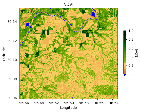

Clip NDVI raster to watersheds

# Define a function to clip the raster with each polygon and return a numpy array
clip_fn = lambda polygon, R: R.rio.clip([polygon.geometry], 
                                        crs=R.rio.crs, 
                                        all_touched=True)

# Apply the function to each row in the GeoDataFrame to create a new 'clipped_raster' column
gdf['clipped_raster'] = gdf.apply(lambda row: clip_fn(row, ndvi), axis=1)

# Inspect resulting GeoDataframe
gdf.head(3)

	CODE_1	NAME_1	AREA	PERIMETER	ACRES	HECTARES_1	DATAID_1	DATACODE_2	geometry	clipped_raster
0	0R1A	R1A	484815.196184	2939.146533	119.800444	48.481520	GIS0321	GIS032	POLYGON ((-96.60663 39.07307, -96.60671 39.073...	[[<xarray.DataArray 'band_data' ()>\narray(nan...
1	R20A	R20A	263364.016292	2509.563160	65.078666	26.336402	GIS0322	GIS032	POLYGON ((-96.60627 39.07163, -96.60627 39.071...	[[<xarray.DataArray 'band_data' ()>\narray(nan...
2	002A	2A	283017.160279	2417.724921	69.935063	28.301716	GIS0323	GIS032	POLYGON ((-96.60294 39.07362, -96.60292 39.073...	[[<xarray.DataArray 'band_data' ()>\narray(nan...

Visualize a specific clipped watershed

We will choose the K1B watershed to show the NDVI for the entire area.

# Select watershed
idx = gdf['NAME_1'] == 'K1B'
row = gdf[idx].index[0]
print(row)

31

# Create figure of selected watershed
fig, ax = plt.subplots(figsize=(6, 6))
gdf.loc[ [row], 'geometry'].boundary.plot(ax=ax, edgecolor='k')
gdf.loc[row, 'clipped_raster'].plot(ax=ax, cmap='ndvi', 
                                    add_colorbar=True, vmin=0.0, vmax=1.0,
                                   cbar_kwargs={'label':'NDVI', 'shrink':0.5})
ax.set_title('K1B')
ax.set_xlabel('Longitude')
ax.set_ylabel('Latitude')

plt.show()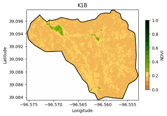

Notice that to plot the boundary of the watershed we had to do: gdf.loc[[row],'geometry'] instead of gdf.loc[row,'geometry']. This is because we need to access the GeoSeries rather than the Shapely polygon.

Compute mean NDVI for each watershed

# Create empty list to append watershed NDVI values
ndvi_avg = []

# Iterate over each watershed
for k,row in gdf.iterrows():
    ndvi_avg.append(np.nanmean(row['clipped_raster'].data))

# Add list of NDVI values to GeoDataframe
gdf.insert(gdf.shape[1]-1, 'ndvi_avg', ndvi_avg)

# Inspect results
gdf.head(3)

	CODE_1	NAME_1	AREA	PERIMETER	ACRES	HECTARES_1	DATAID_1	DATACODE_2	geometry	ndvi_avg	clipped_raster
0	0R1A	R1A	484815.196184	2939.146533	119.800444	48.481520	GIS0321	GIS032	POLYGON ((-96.60663 39.07307, -96.60671 39.073...	0.187059	[[<xarray.DataArray 'band_data' ()>\narray(nan...
1	R20A	R20A	263364.016292	2509.563160	65.078666	26.336402	GIS0322	GIS032	POLYGON ((-96.60627 39.07163, -96.60627 39.071...	0.196402	[[<xarray.DataArray 'band_data' ()>\narray(nan...
2	002A	2A	283017.160279	2417.724921	69.935063	28.301716	GIS0323	GIS032	POLYGON ((-96.60294 39.07362, -96.60292 39.073...	0.173563	[[<xarray.DataArray 'band_data' ()>\narray(nan...

Create static map

# Create figure with mean NDVI values for each watershed
gdf.plot(column='ndvi_avg', edgecolor='k', cmap='ndvi', 
         legend=True, vmin=0.0, vmax=1.0, legend_kwds={'label':'NDVI', 'shrink':0.5})
plt.title('Konza Prairie Mean NDVI April 2024')
plt.xlabel('Longitude')
plt.ylabel('Latitude')
#plt.savefig('Konza Mean NDVI April 2024.jpg', dpi=300)
plt.show()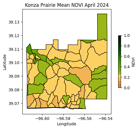

Create interactive map

# Create interactive map
gdf.iloc[:,:-1].explore(column='ndvi_avg', k=10, cmap='ndvi',
                        style_kwds={'stroke':True,'color':'black','width':1},
                        legend_kwds={'caption':'NDVI'})

Make this Notebook Trusted to load map: File -> Trust Notebook