89  Built-in spatial interpolators

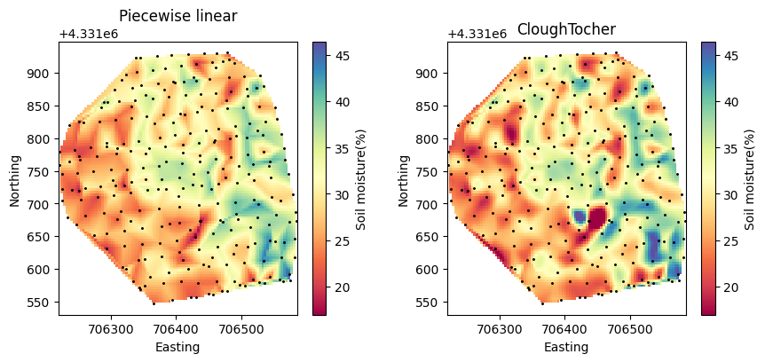
Spatial interpolation is a technique where regaurly spaced or irregularly spaced data points distributed across a region are used to estimate the value at unsampled points. In this tutorial, we will use Scipy’s LinearNDInterpolator and CloughTocher2DInterpolator functions for approximating soil moisture values at unsampled locations between non-regularly spaced observations.

The LinearNDInterpolator consists of a piece-wise linear interpolation to estimate values at arbitrary locations within the convex hull formed by the input data points.

The CloughTocher2DInterpolator uses a triangular interpolation, which provides a smoother and potentially more accurate representation of the data’s spatial variation. This method constructs a continuous surface over the input data by fitting quadratic surfaces for each triangle formed by the data points.

# Import modules
import numpy as np
import pandas as pd
import geopandas as gpd
import matplotlib.pyplot as plt
from scipy.interpolate import CloughTocher2DInterpolator, LinearNDInterpolator

# Define coordiante reference systems
crs_utm = 32614 # UTM Zone 14
crs_wgs = 4326 # WGS84

# Read dataset
df = pd.read_csv('../datasets/spatial/soil_moisture_surveys/kona_15_jul_2019.csv')

# Inspect a few rows
df.head(3)

	TimeStamp	Record	Zone	Latitude	Longitude	Moisture	Period	Attenuation	Permittivity	Probe Model	Sensor
0	7/15/2019 7:15	320	ZONE 00001	39.11060	-96.61089	38.88	1.6988	1.8181	23.8419	CD659 12cm rods	3543
1	7/15/2019 7:17	321	ZONE 00001, ZONE 00011	39.11058	-96.61116	41.71	1.7474	1.8310	26.7794	CD659 12cm rods	3543
2	7/15/2019 7:17	322	ZONE 00001, ZONE 00011	39.11055	-96.61146	40.59	1.7271	1.7911	25.5712	CD659 12cm rods	3543

# Drop lines with NaN in 'Moisture' column
df.dropna(subset='Moisture', inplace=True)
df.reset_index(drop=True, inplace=True)

# Convert Dataframe to GeoDataframe
gdf = gpd.GeoDataFrame(df)

# Add Point geometry from lat and long values
gdf['points'] = gpd.points_from_xy(gdf['Longitude'], gdf['Latitude'])
gdf.set_geometry('points', drop=True, inplace=True, crs=crs_wgs)

# Inspect spatial data
plt.figure(figsize=(5,4))
plt.title('KONA field')
gdf.plot(ax=plt.gca(), edgecolor='k', marker='.', s=80, column='Moisture',
         cmap='Spectral', scheme='equal_interval', k=8, legend=True,
         legend_kwds={'loc':'upper left',
                      'bbox_to_anchor':(1.05,1),
                      'title':'Soil moisture (%)'})
plt.xlabel('Longitude')
plt.ylabel('Latitude')
plt.show()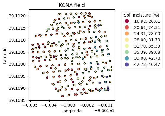

# Convert point coordinates to UTM, so that we can work in meters
# to compute distances within the field
gdf.to_crs(crs=crs_utm, inplace=True)

# Get values of longitude (x) and latitude (y) in meters
x = gdf['geometry'].x.values
y = gdf['geometry'].y.values
z = gdf['Moisture'].values

# Create tuple of points
points = (x, y)

# Generate grid
x_vec = np.linspace(x.min(), x.max(), num=100)
y_vec = np.linspace(y.min(), y.max(), num=100)

# Create grid
X_grid, Y_grid = np.meshgrid(x_vec, y_vec)
print(X_grid.shape)

(100, 100)

# Interpolation using LinearNDInterpolator
NDinterp = LinearNDInterpolator(list(zip(x, y)), z)
Z_grid_NDinterp = NDinterp(X_grid, Y_grid)

# Interpolation using CloughTocher
CTinterp = CloughTocher2DInterpolator(list(zip(x, y)), z)
Z_grid_CTinterp = CTinterp(X_grid, Y_grid)

plt.figure(figsize=(10,4))

plt.subplot(1,2,1)
plt.title('Piecewise linear')
p1 = plt.pcolormesh(X_grid, Y_grid, Z_grid_NDinterp, 
               cmap='Spectral', vmin=z.min(), vmax=z.max())
plt.scatter(x, y, color='k', marker='.', s=5)
plt.colorbar(p1, label='Soil moisture(%)')
plt.axis("equal")
plt.xlabel('Easting')
plt.ylabel('Northing')

plt.subplot(1,2,2)
plt.title('CloughTocher')
p2 = plt.pcolormesh(X_grid, Y_grid, Z_grid_CTinterp, 
               cmap='Spectral', vmin=z.min(), vmax=z.max())
plt.scatter(x, y, color='k', marker='.', s=5)
plt.colorbar(p2, label='Soil moisture(%)')
plt.axis("equal")
plt.xlabel('Easting')
plt.ylabel('Northing')

plt.subplots_adjust(wspace=0.3)
plt.show()