HP-SDI12-NANO heat-pulse sensor · background chapter · September 2026
How the heat-pulse sensor works
An introductory chapter on the electronics and the heat-transfer model behind the digital twin, written for a first-year electrical-engineering student and for anyone coming from agronomy or soil science.
Andres Patrignani, Garrett Peterson, Gerard Kluitenberg, Eduardo Santos, and Bala Natarajan
AI disclosure. This chapter was drafted with Claude Opus 5.5 (Anthropic), an AI assistant, in September 2026. Working from the authors’ instructions, peer-reviewed articles provided by the authors, team meeting notes, correspondence between team members, the sensor design files, the digital twin, and its own general knowledge, it wrote the text, wrote the Python code that draws the figures, and ran the calculations. Most calculations were also implemented in a Jupyter notebook for reproducibility and scrutiny by the authors. The authors directed the work, reviewed and edited the content, and are responsible for it.
What you will learn
How a heat-pulse sensor measures soil thermal properties
Basic electricity: voltage, current, resistance and capacitors
How the sensor turns temperature into a number
How a heat-flow model estimates thermal properties and water content
How design choices affect the measurement
All numbers come from the current sensor design and its digital twin.
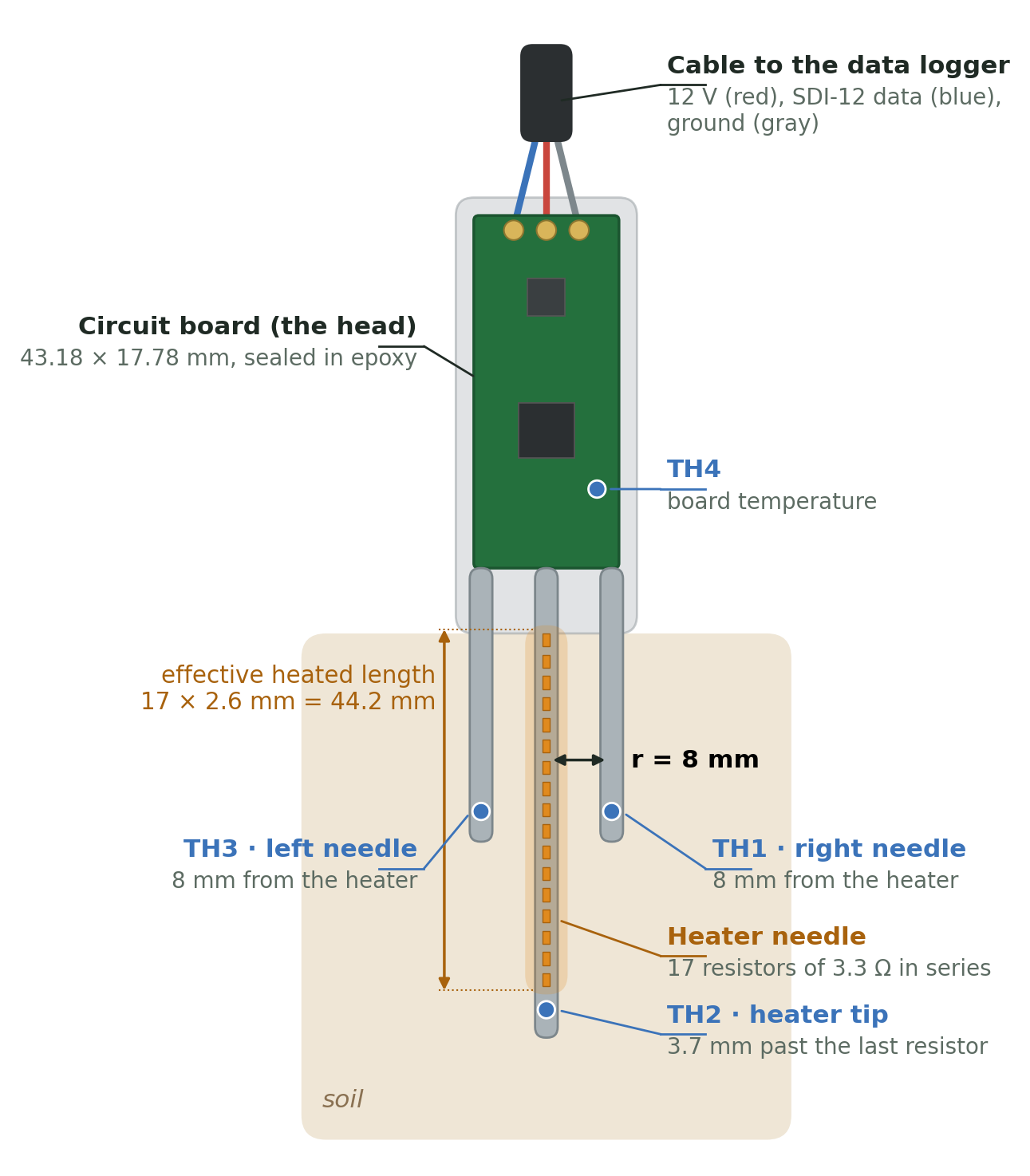
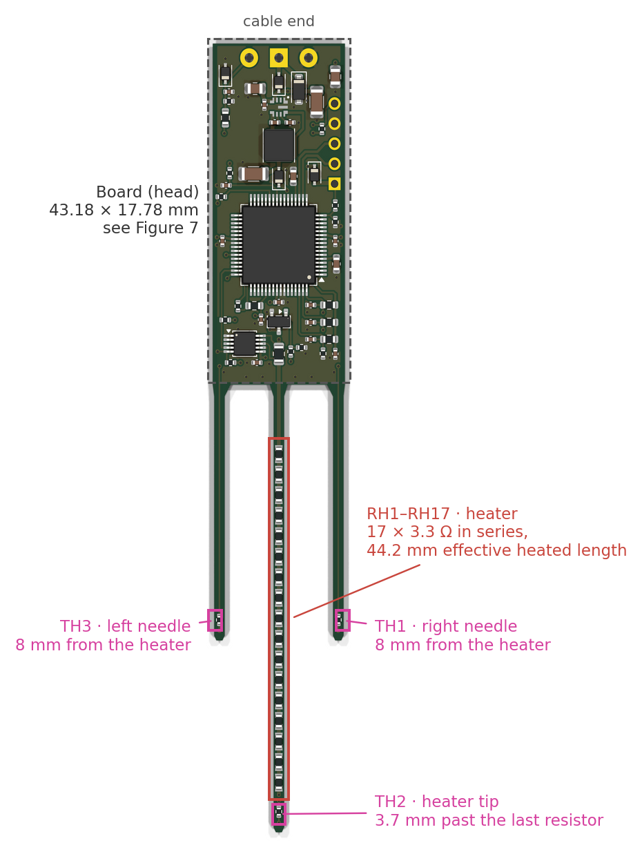
The sensor has a small circuit board (the "head") and three thin needles that go into the soil. The center needle is a heater: seventeen tiny 3.3 Ω resistors in a row. The two side needles carry thermometers (thermistors TH1 and TH3), 8 mm away from the heater. A third thermistor, TH2, sits at the tip of the heater needle, and TH4 sits on the board to report the board's own temperature.
Figure 1. The sensor, drawn to scale (millimeters): cable end up, needles down, seen from the board's top face, the way the website draws it. The 12-gauge steel needles (2.77 mm across) slide over the board's three prongs. TH1 and TH3 sit halfway along the heated section, 8 mm from the heater; TH2 sits just past the last heater resistor. Left and right are as seen in this view.
A data logger asks for each measurement over a single data wire, using SDI-12, a standard way for environmental sensors to talk to loggers. One measurement goes like this (Figure 1 shows where each part sits):
Background (10 s). Record the soil temperature before heating, so we can subtract it later.
Heating (15 s). Push about 2 W through the heater. That is roughly the power of a small flashlight bulb, spread along 44 mm of needle.
Cooling (150 s). Keep recording while the heat spreads outward. The side needles warm up by about half a degree, peak about 23 s after the heater switches off, and slowly cool.
Analysis. How high the side-needle curve rises tells us how much heat the soil can store (its heat capacity). How fast the peak arrives tells us how fast a temperature change spreads through it (its diffusivity). Together they give the thermal conductivity, and the heat capacity gives the water content, because water stores far more heat than soil minerals or air.
Analogy. Drop a spoonful of dye into still water and watch a spot 8 mm away. In thick syrup the color arrives late and stays concentrated; in water it arrives quickly and fades fast. The heat pulse is the dye, the soil is the liquid, and the side thermistor is your eye. The one difference: we know exactly how much "dye" (energy, in joules) we released, because we measure the heater power.
Two pieces of engineering make this work: an electronic circuit that measures temperature to a few thousandths of a degree (Sections 2 and 3), and a physical model that converts the temperature curve into soil properties (Sections 4 to 6).
2. Electricity for soil scientists
2.1 Voltage, current, resistance
Three quantities describe almost everything on this board:
Quantity
Symbol · unit
What it is
Water analogy
Voltage
\(V\) · volt (V)
The "push" that drives charge, always measured between two points
Water pressure (height difference between two tanks)
Current
\(I\) · ampere (A)
How much charge flows per second
Flow rate (liters per second)
Resistance
\(R\) · ohm (Ω)
How strongly a part opposes the flow
A narrow section of pipe
Power
\(P\) · watt (W)
Energy converted per second (in a resistor: to heat)
Pressure × flow: the work the water does
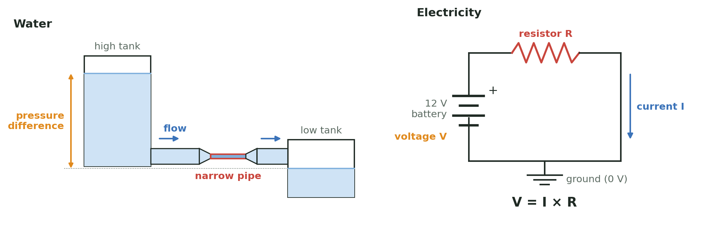
Figure 2 pictures these quantities with water. Handy prefixes: 1 mA = 0.001 A, 1 µA = 0.000001 A, 1 kΩ = 1000 Ω, 1 mW = 0.001 W. Ground (GND) is simply the point we call 0 V; every other voltage on the board is measured from it, just as elevations are measured from sea level.
Figure 2. The water analogy, side by side with the circuit it stands for. The height difference between the tanks drives the flow, as the battery's voltage drives the current; the narrow pipe limits the flow and is where the energy is spent, as the resistor limits the current and turns energy into heat; the low tank is ground. This is exactly how the heater needle works.
2.2 Ohm's law and power, with the heater
For a resistor, current is proportional to voltage:
$$ V = I\,R \qquad\Longleftrightarrow\qquad I = \frac{V}{R} \qquad\Longleftrightarrow\qquad R = \frac{V}{I}$$
and the power it turns into heat is
$$ P = V\,I = I^2 R = \frac{V^2}{R}. $$
Worked example: the heater. Seventeen 3.3 Ω resistors in a row (in series, one after the other) add up: \(R_\text{heater} = 17 \times 3.3 = 56.1\ \Omega\). If the full 12 V battery sat across the heater, the current would be \(12/56.1 = 0.214\) A. In reality a few other things are in the same loop, and each takes its share:
Part of the loop
Resistance or drop
Input diode D1 (protects against a reversed battery)
≈ 0.35 V drop
5 m of 22 AWG cable, out and back (10 m of wire)
≈ 0.53 Ω
Current-sense resistor R5 (the INA226 measures the current here)
So the heater gets \(P = I^2R = 0.2045^2 \times 56.1 = 2.35\) W while it is on, and each little resistor gets \(0.2045^2 \times 3.3 = 0.138\) W, well under its 0.33 W rating.
PWM: turning a heater "down" with a switch. We cannot easily change the battery voltage, but we can switch the heater on and off very fast. The processor will switch Q1 100 times per second and keeps it on 85% of each cycle (the duty cycle). The soil cannot feel 100 flickers per second, so it sees the average: \(0.85 \times 2.35 = 1.99\) W. Over a 15 s pulse the energy is \(E = P\,t = 1.99 \times 15 \approx 29.9\) J. That energy divided by the heater's effective length, \(29.9\ \text{J} / 0.0442\ \text{m} \approx 677\) J per meter, is the key input to the soil model in Section 5.
2.3 Series resistors and the voltage divider
Put two resistors in series between a voltage \(V_\text{top}\) and ground. The same current flows through both, \(I = V_\text{top}/(R_1+R_2)\), so the voltage at the point between them is
This is the voltage divider, and it is the heart of the temperature measurement: if \(R_2\) changes with temperature, so does \(V_\text{mid}\). If \(R_1 = R_2\), the midpoint sits at exactly half of \(V_\text{top}\).
Analogy. Water flows down a hill through two stretches of narrow pipe. The pressure halfway down depends on how the total "resistance" is split between the upper and lower stretch. Make the lower stretch narrower and more of the pressure drop happens there, so the midpoint pressure rises.
2.4 Capacitors and the RC time constant
A capacitor stores electric charge, like a small bucket. Its size, the capacitance \(C\), is measured in farads (F); ours are 100 nF (0.0000001 F) and 1 µF. The charge it holds is \(Q = C\,V\): a bigger bucket, or a fuller one, holds more.
A capacitor does two useful jobs: it smooths (it absorbs sudden spikes and fills in brief dips, like a water tower on a town's water line), and together with a resistor it sets a delay. If you fill a capacitor through a resistor \(R\) from a voltage \(V_0\), it charges along
The time constant \(\tau\) is the whole story: after one \(\tau\) the capacitor is 63% full, after 5\(\tau\) it is 99.3% full, and after 10\(\tau\) it is within 0.005% of its final value. Example: 1.5 kΩ and 1 µF give \(\tau = 1500 \times 0.000001 = 1.5\) ms.
Analogy. Filling a bathtub through a garden hose. The tub is the capacitor, the hose is the resistor. A thinner hose (more R) or a bigger tub (more C) means a longer wait. The tub fills fast at first and slows as it nears full, because the pressure difference that drives the flow shrinks. That is the exponential curve above.
3. The thermistor circuit, part by part
Figure 3. One of the four thermistor channels. Pin D4 powers VREF through R11; C13 holds VREF steady. VREF feeds the reference resistor R21 on top and the thermistor TH1 below it, and the same VREF is the processor's measuring "ruler" (AREF). C21 steadies the node that the processor reads.
3.1 The thermistor
A thermistor is a resistor made to change its resistance with temperature. Ours are "NTC" (negative temperature coefficient): warmer means lower resistance. At 25 °C it is nominally 10 kΩ (±1%). The standard "beta" equation describes it:
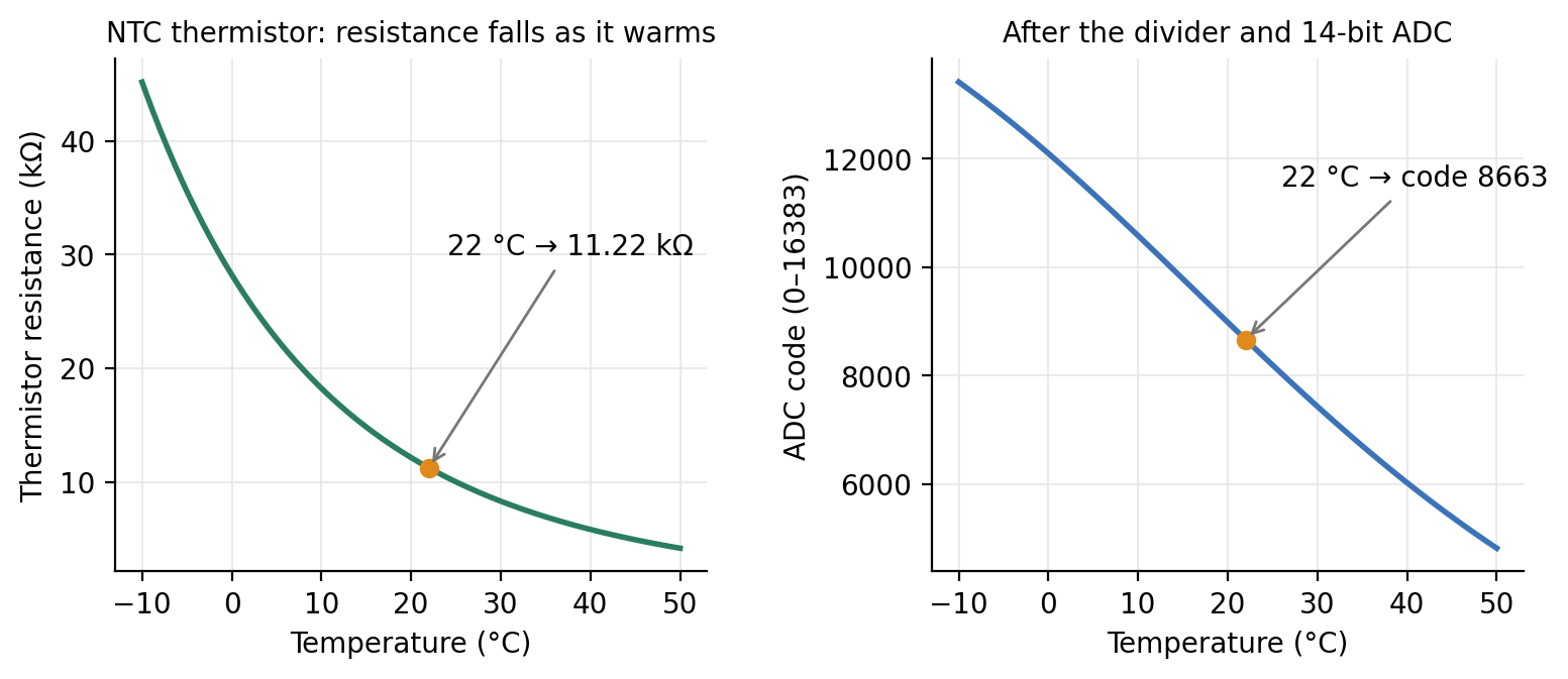
with \(T\) in kelvin (°C + 273.15). Near room temperature the resistance changes by about \(\beta/T^2 \approx 3.8\%\) per degree, which is large; that is why thermistors are good at sensing small temperature changes (Figure 4, left).
Figure 4. Left: resistance of the thermistor. At 22 °C it is 11.22 kΩ. Right: the number the processor sees after the divider and the analog-to-digital converter (Sections 3.2 and 3.3).
3.2 Why a reference resistor (R21–R24)?
The processor cannot measure resistance. It can only measure voltage. The reference resistor turns a resistance into a voltage by forming a divider with the thermistor (Section 2.3; Figure 3):
Example at 22 °C: \(R_\text{NTC} = 11.22\) kΩ, \(R_\text{ref} = 10\) kΩ, \(V_\text{REF} = 3.53\) V, so the current is \(3.53/21.22\ \text{k}\Omega = 166\ \mu\text{A}\) and \(V_\text{node} = 3.53 \times 11.22/21.22 = 1.87\) V. Warm the soil and the thermistor's resistance drops, so the node voltage drops.
Why 10 kΩ? Choosing the reference equal to the thermistor's nominal value puts the node near half of VREF, where the divider is most sensitive to small changes. Why 0.1% precision and 25 ppm/°C? Any error in the reference resistor looks exactly like a temperature error. A 1% resistor would shift the reading by about 1%/3.8% ≈ 0.26 °C; the 0.1% part keeps that below 0.03 °C, and its low temperature coefficient keeps it from drifting as the board warms or cools. For the soil properties, what matters is the temperature rise, and a fixed offset cancels when the background is subtracted: a 1% reference error changes the rise by only about 0.2%. The thermistor's \(\beta\) value is different: an error in \(\beta\) scales every rise, and therefore \(\lambda\) and \(C\), one for one.
Does the divider linearize the thermistor? Only as a side effect. The right panel of Figure 4 is not an approximation of the left one: it is the exact result, code = 16384 × R / (R + 10 kΩ). The fraction R / (R + Rref) flattens toward 1 when the thermistor resistance is large and toward 0 when it is small, which counteracts the thermistor’s steep exponential curve. The result is an S-shaped curve that is nearly straight around the temperature where the thermistor equals the reference resistor (25 °C here) and bends more toward cold and hot temperatures. The processor never uses a straight-line approximation: it inverts the exact divider and beta equations (Section 3.3), which costs only a few lines of arithmetic. What the divider’s shape buys is nearly even resolution across the range of soil temperatures:
Temperature
Thermistor
ADC code
Codes per °C
°C per code
-10 °C
45.2 kΩ
13414
119
0.0084 °C
0 °C
28.2 kΩ
12098
143
0.0070 °C
10 °C
18.2 kΩ
10581
158
0.0063 °C
22 °C
11.2 kΩ
8663
158
0.0063 °C
25 °C
10.0 kΩ
8192
156
0.0064 °C
40 °C
5.8 kΩ
6021
131
0.0076 °C
50 °C
4.2 kΩ
4813
110
0.0091 °C
60 °C
3.0 kΩ
3819
89
0.0112 °C
Near-surface soil can reach 50–60 °C in summer, especially while the heater is on. Even at 60 °C one code is about 0.011 °C, about 45 times finer than the half-degree signal. A smaller reference resistor would move the flattest part of the curve to warmer temperatures: with 6.8 kΩ, the value matching the thermistor at about 35 °C, resolution at 60 °C improves by about 20% but is about 13% worse at 10 °C, and the dividers draw more current, which lowers VREF and adds a little self-heating. Because noise, not the number of ADC steps, will limit the measurement, 10 kΩ remains a sound choice for the whole 0–60 °C range.
3.3 From voltage to a number: the ADC
The processor's analog-to-digital converter (ADC) compares the input voltage with a reference voltage and reports a whole number, the code. With 14 bits there are \(2^{14} = 16384\) steps:
Here is the trick in this design: the ADC's reference (AREF) is connected to the same VREF that feeds the dividers. Substitute the divider equation and VREF cancels:
Analogy: a stretchy ruler. Measure a rubber band with a ruler printed on the same rubber. If both stretch together, the reading does not change. This is called a ratiometric measurement: VREF can sag or drift a little and the temperature reading stays the same, because the "ruler" (AREF) and the "object" (the divider) move together.
Worked example. At 22 °C: code = 16384 × 11.22/21.22 = 8663. Going back: \(R = 10\ \text{k}\Omega \times 8663/(16384-8663) = 11.22\) kΩ, and inverting the beta equation,
How fine is the measurement? Near 22 °C the code changes by about 158 codes per °C, so one code is about 0.006 °C. The planned firmware averages 64 readings per sample (the twin assumes this), which reduces random noise further. The signal we want, the side-needle rise, is about 0.5 °C, or roughly 80 codes. The real limits are noise, thermistor calibration and the reference resistor, not the number of steps.
3.4 Why the thermistors are switched on only to read
Current through a thermistor heats it. This self-heating is a real problem when the signal is half a degree. During a reading the thermistor carries 166 µA with 1.87 V across it:
$$ P = V I = 1.87\ \text{V} \times 166\ \mu\text{A} \approx 0.31\ \text{mW}. $$
The maker quotes a "dissipation constant" of about 1 mW/°C in still air, so 0.31 mW would warm the thermistor by about 0.3 °C; in epoxy and soil heat escapes more easily, so the real warming is smaller. Left on all the time, that would be a steady warming comparable to the signal. A perfectly steady offset would cancel when the background is subtracted, but this one would not be steady: it depends on how well the thermistor is coupled to the soil, which changes with moisture, and it warms the very spot being measured. So pin D4 powers the whole thermistor network only 20 ms out of every second (2%). The average heating power drops to about 6 µW, and the self-heating to a few thousandths of a degree. It also saves battery.
Analogy. Checking whether bread is done by touching it: a quick tap tells you the temperature; holding your hand on it warms the bread. The thermistors get a quick tap once per second.
3.5 Why R11 (1.5 kΩ)?
Pin D4 is a processor output, and processor pins are delicate: the RA4M1 data sheet lists 4 mA per pin for this port (Arduino's Nano R4 documentation quotes up to 8 mA; the design uses the more conservative data-sheet value). When D4 switches on, C13 is empty and behaves for an instant like a short circuit to ground. Without a resistor the pin would try to deliver a large current. R11 limits it by Ohm's law:
(An earlier version used 330 Ω, which would have allowed about 14 mA; that is why it was changed.) Once C13 is charged, R11 carries the steady current of the four dividers plus the ADC reference, about 0.8 mA. That current makes a voltage drop across R11, \(1500\ \Omega \times 0.8\ \text{mA} \approx 1.2\) V, which is why VREF settles near 3.5 V rather than 4.75 V. Thanks to the ratiometric trick, that lower value does not matter.
3.6 Why C13 and C21–C24?
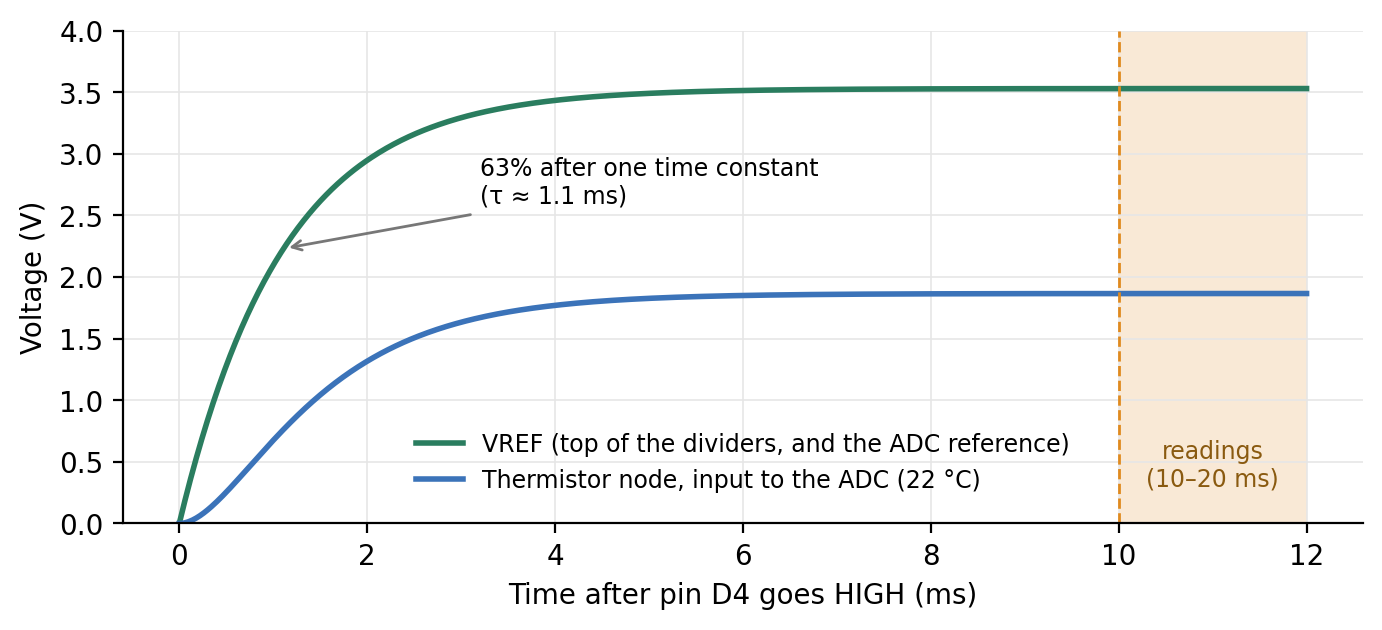
C13 (1 µF) holds VREF steady. The ADC draws small, quick sips of current from its reference while it converts. Without a local "bucket," each sip would dent VREF through R11. C13 supplies the sips and refills between them. With R11 it charges with a time constant of about 1.1 ms (R11 in parallel with the divider load, times 1 µF).
C21–C24 (100 nF each) hold each thermistor node steady. Three reasons:
The ADC takes a gulp. Inside the ADC, a tiny capacitor is connected to the input for a moment and must be charged to the input voltage. Through 5 kΩ of divider resistance, that gulp would pull the voltage down briefly. The 100 nF capacitor is thousands of times larger than the ADC's internal one, so it supplies the gulp with almost no change in voltage.
The needle wires are antennas. The thermistor wires run 30 to 55 mm down the needles, right next to a heater that switches 100 times per second. They pick up electrical noise. The capacitor, together with the divider resistance, forms a filter that smooths out fast disturbances while passing the slow temperature signal.
A known, short settling time. Each node settles with \(\tau = (10\ \text{k}\Omega \parallel R_\text{NTC}) \times 100\ \text{nF} \approx 5.3\ \text{k}\Omega \times 100\ \text{nF} = 0.53\) ms. The planned firmware waits 10 ms before reading. That is nearly 19 of the node's own time constants, but the node also follows VREF, which settles more slowly (about 9 of its time constants in 10 ms). The node-to-VREF ratio is within about one ADC step at the first reading and closer on average, and the small remainder is the same every second, so it cancels when the background is subtracted.
Why not bigger capacitors? Bigger capacitors would smooth more but take longer to charge, so pin D4 would have to stay on longer (more self-heating) and the network would need longer to discharge between readings. The values are a balance between steadiness and speed.
3.7 One reading, millisecond by millisecond
This is the planned sequence that the twin simulates (Figure 5); the firmware is still to be written.
Figure 5. After pin D4 goes HIGH, VREF rises with a time constant of about 1.1 ms, and the thermistor node follows a little later through its own 0.53 ms filter. Both are flat long before the readings start at 10 ms. At 20 ms pin D4 goes LOW and everything discharges until the next second.
Time
What happens
0 ms
Pin D4 goes HIGH. R11 limits the inrush into C13 to 3.2 mA.
0–10 ms
VREF and the four thermistor nodes charge and settle (about 9 and 19 time constants).
10–20 ms
The ADC takes 64 readings of each of A0–A3 and averages them.
20 ms
Pin D4 goes LOW; the network discharges. The thermistors rest for the remaining 980 ms.
every 1 s
Repeat, through the background, heating and cooling phases.
3.8 Where the parts sit on the board
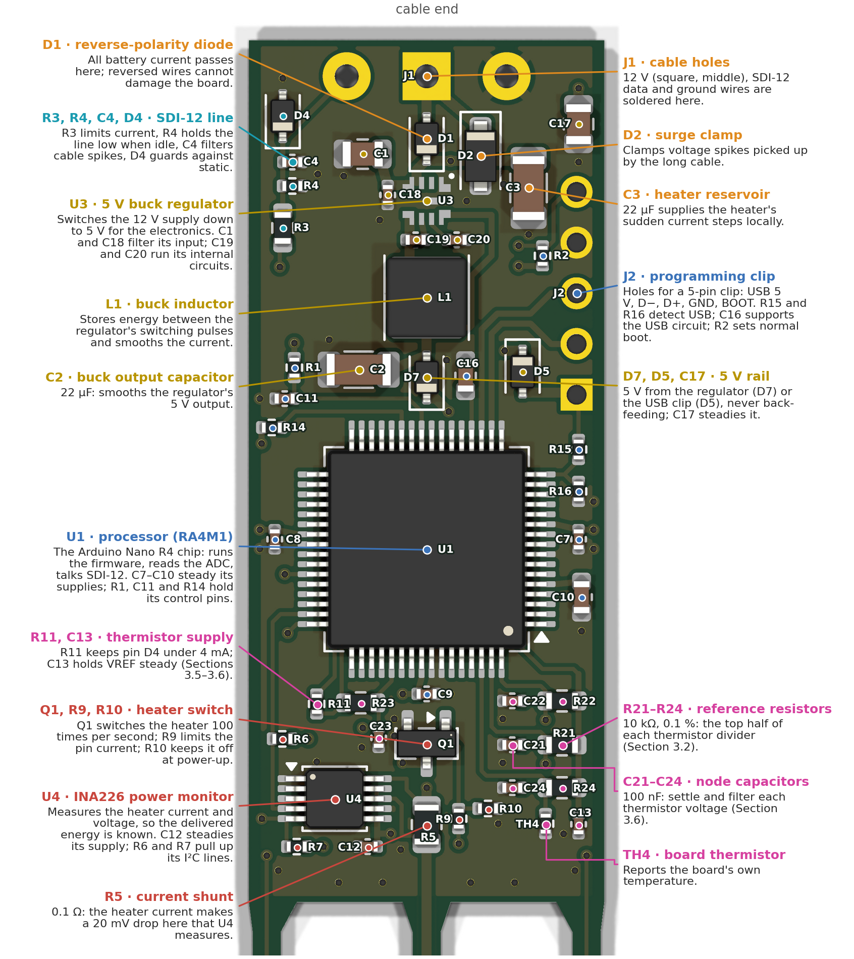
Everything in Sections 2 and 3 is a real part you can find on the board. Figure 6 shows the whole sensor as KiCad renders it, turned the way the website draws it: cable end up, needles down, seen from the top face (so TH1 is on the right). Figure 7 zooms in on the head. Every part is marked with a dot and its name, each color is one job, and the text beside each group says in a sentence what it does and which section explains it. Appendix A lists every part with its manufacturer, part number and specifications.
Color
Job
Where the theory is
Orange
Power coming in from the battery, and its protection
Section 2.2 (Ohm's law around the heater loop)
Gold
Making and distributing the 5 V for the electronics
Section 2.4 (capacitors as buckets)
Blue
The processor and its programming holes
Section 3.3 (the ADC lives inside U1)
Teal
The SDI-12 line to the data logger
Section 1; tour step 9 on the website
Pink
Temperature measurement: the thermistor circuit of Figure 3
Sections 3.1–3.7
Red
The heater: switching it and measuring the power it delivers
Sections 2.2 and 5.5 (\(q'\) comes from U4's measurement)
Figure 6. The whole sensor (KiCad render of the current board). The heater's 17 resistors run down the center needle; TH1 and TH3 sit on the side needles halfway along the heated section, and TH2 sits just past the last resistor. The dashed box is the head, enlarged in Figure 7.Figure 7. The head, part by part. Every part is marked with a dot and its name (the names are the ones used throughout this chapter and in Appendix A). Dots of one color belong to one job (the colors follow the table in Section 3.8); the line from each description ends on the group's main part, the larger dot. TH1–TH3 and the heater resistors sit on the needles (Figure 6). The measurement parts (pink) sit together near the needles, away from the switching regulator at the cable end, and the parts that warm up in use (U1, U3, L1, D1, D7, R5, Q1) sit on the board’s center line, so they warm both side needles equally.
4. Heat in soil
Three properties describe how a material handles heat:
Property
Symbol · unit
Meaning
Analogy
Thermal conductivity
\(\lambda\) · W m⁻¹ K⁻¹
How easily heat flows through it
How wide the pipes are
Volumetric heat capacity
\(C\) · J m⁻³ K⁻¹ (MJ m⁻³ K⁻¹)
Energy needed to warm 1 m³ by 1 °C
How big each bucket is
Thermal diffusivity
\(\alpha = \lambda/C\) · m² s⁻¹ (mm² s⁻¹)
How fast a temperature change spreads
Wide pipes into small buckets: news travels fast
Soil is a mix of minerals, organic matter, water and air, and the mix sets the properties:
Material
\(\lambda\) (W m⁻¹ K⁻¹)
\(C\) (MJ m⁻³ K⁻¹)
Water
0.6
4.18
Air
0.025
0.0012
Quartz
≈ 8
≈ 2.0
Other soil minerals
≈ 2–3
≈ 2.0
Dry soil (typical)
0.2–0.5
1.0–1.4
Moist soil (typical)
1.0–2.0
2.0–3.2
The key fact for water content: water has twice the heat capacity of minerals and three thousand times that of air. When a soil gains water, the water replaces air, and the heat capacity climbs linearly with the water content. Measure \(C\), and you can back out the water content (Section 5.6).
5. The line-source model
5.1 The heat equation
Heat flows from warm to cold at a rate proportional to the temperature gradient (Fourier's law), and energy is conserved. Combining the two gives the heat equation:
In words: a spot warms up if it is colder than the average of its surroundings, and the rate is set by the diffusivity. For a long, straight heater it is natural to use distance from the heater, \(r\), as the coordinate; if nothing changes along the heater's length, the equation becomes
The extra \(1/r\) term appears because heat spreads over ever-larger rings: a ring twice as far away has twice the circumference to warm.
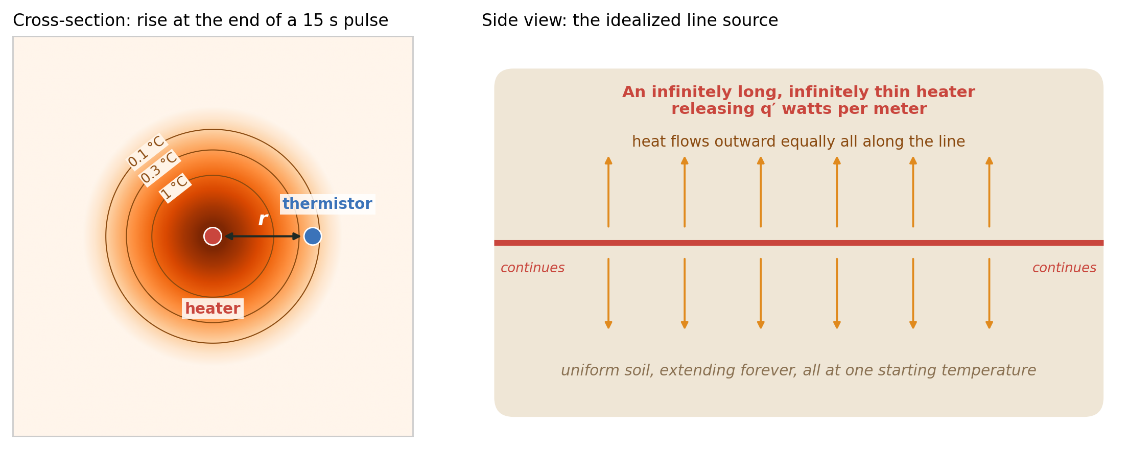
Figure 8. The idealized picture behind the line-source model. Left: temperature rise in a cross-section around the line at the end of a 15 s pulse (medium soil, rings at 0.1, 0.3 and 1 °C); the thermistor, 8 mm away, has warmed by about 0.13 °C so far and keeps warming after the heater stops. Right: the assumptions of Section 5.2 in one picture.
5.2 Assumptions and boundary conditions
To solve the equation we must say what the world looks like (Figure 8). The classic dual-probe analysis (Campbell et al. 1991, who treated the heat pulse as instantaneous; Kluitenberg et al. 1993 and Bristow et al. 1994, who included its finite duration) assumes:
Geometry: the heater is an infinitely long, infinitely thin line.
Medium: the soil is uniform (homogeneous and the same in every direction) and extends forever in every direction.
Initial condition: everything starts at the same temperature; we work with the rise \(\Delta T = T - T_0\), which starts at zero everywhere.
Far-field boundary condition: far away the soil never feels the heater, \(\Delta T \to 0\) as \(r \to \infty\).
Source condition: the line releases a constant power per meter, \(q'\), from time 0 to time \(t_0\), then stops.
Everything else is ignored: the needles' own size and heat storage, the epoxy, contact resistance between needle and soil, the soil surface, water moving in response to heat, and properties changing with temperature.
5.3 Continuous and pulsed line source
If the line heats forever, the solution (Carslaw and Jaeger 1959; Blackwell 1954) is
where \(E_1\) is the exponential integral, \(E_1(x) = \int_x^\infty \frac{e^{-u}}{u}\,du\). You do not need to compute it by hand: it is built into scientific libraries (for example scipy.special.exp1 in Python or expint in MATLAB), but not into common spreadsheets or data-logger function libraries; Knight and Kluitenberg (2004) give a simple polynomial approximation for those cases. All you need to know is that it is large for small arguments (long times, short distances) and falls quickly to zero for large ones. The group \(r^2/(4\alpha t)\) is a natural "clock": the heat front reaches a distance \(r\) at a time of order \(r^2/(4\alpha)\), which for our 8 mm and a typical soil is about 30 s.
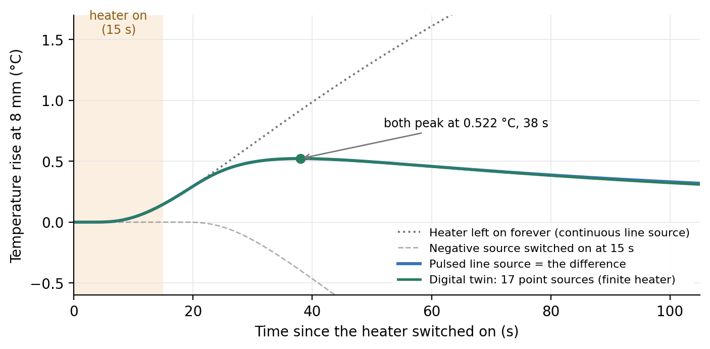
Switching off: superposition. The heat equation is linear, so solutions can be added. Turning the heater off at \(t_0\) is the same as leaving it on and adding a second, negative heater that starts at \(t_0\):
Analogy. Stopping a faucet is equivalent to leaving it running and opening a drain of the same size underneath. Mathematically this is simpler, because both the faucet and the drain have the same, known behavior.
Figure 9. The pulsed line source (blue) is the continuous solution (dotted) plus a negative source switched on at 15 s (dashed, already drawn negative). The green curve is what the digital twin computes with the real, finite heater (Section 6). With the heater's power spread over its effective length (Section 5.5), the two curves peak at the same height and time; they part only late in the tail (Section 6.3).
5.4 Reading soil properties from the peak
The side-needle curve rises, peaks at a time \(t_m\) with height \(\Delta T_m\), and falls. Setting the time derivative of the pulsed solution to zero gives a formula for the diffusivity from the peak time alone (Bristow et al. 1994):
The intuition, from a very short pulse. If all the energy \(Q' = q' t_0\) (joules per meter) were released at once, the solution would be \(\Delta T = \frac{Q'}{4\pi\lambda t}\exp\!\left(-\frac{r^2}{4\alpha t}\right)\); its peak comes at \(t_m = r^2/(4\alpha)\) and has height (Campbell et al. 1991)
Read it like this: the pulse of energy spreads into a cylinder of soil of roughly radius \(r\) (cross-section \(\pi r^2\)); the temperature rise is energy divided by (volume × heat capacity), and the factor \(1/e\) (with \(e \approx 2.718\)) is how far down the bell-shaped temperature profile the thermistor sits at that moment: at \(t_m\) the profile has \(\exp(-r^2/4\alpha t_m) = e^{-1}\) at distance \(r\). A soil that stores more heat (wetter) shows a smaller peak. The formula also shows why the spacing matters so much: \(C\) depends on \(r^2\), so a 1% error in spacing becomes a 2% error in heat capacity.
5.5 Worked example: Hodgeman 20 cm, 33 kPa
This is the twin's default soil, a silty clay loam core from the Kansas Mesonet soil database (Parker et al. 2022) whose KD2 Pro readings are \(\lambda = 1.283\) W m⁻¹ K⁻¹ and \(C = 2.345\) MJ m⁻³ K⁻¹ (so \(\alpha = 0.547\) mm² s⁻¹).
Step
Calculation
Result
Heater power (average)
\(0.85 \times 2.346\) W
1.994 W
Effective heated length
17 resistors × 2.6 mm (see the note below)
44.2 mm
Power per meter
\(q' = 1.994 / 0.0442\)
45.11 W m⁻¹
Energy per meter
\(Q' = q' t_0 = 45.11 \times 15\)
677 J m⁻¹
Predicted peak (ideal line)
pulsed equation, \(r\) = 8 mm
0.522 °C at 38.0 s
Why 44.2 mm and not 43.2 mm? Measured from the first resistor's outer end to the last one's, the 17 resistors span 43.2 mm. But each resistor stands for one 2.6 mm stretch of an evenly heated line: seventeen stretches of 2.6 mm make 44.2 mm. That is the length the line-source model needs. Using 43.2 mm overstates \(q'\) by 2.3%, and \(\lambda\) and \(C\) come out 2.3% high (Section 6.3).
Now pretend we measured that curve and want the soil back. With \(t_m = 38\) s, \(t_0 = 15\) s and \(r = 0.008\) m:
We recover the soil to within rounding, as we should when the data follow the model perfectly. The short-pulse shortcut gives \(C = 677/(2.718 \times \pi \times 0.008^2 \times 0.5221) = 2.37\) MJ m⁻³ K⁻¹, only 1% off, a good sanity check you can do on a calculator.
How sensitive is this? Two small errors, worked out for this example:
Peak time off by 1 s (37 or 39 s instead of 38 s): \(\alpha\) and \(\lambda\) change by about ±3.5%, but \(C\) changes by less than 0.1%. The peak time sets the diffusivity; the conductivity follows it, and the heat capacity, which depends mostly on the peak height, hardly moves.
Spacing off by 0.1 mm (analysis assumes 8.1 mm, needles really 8.0 mm): \(\alpha\) comes out 2.5% high and \(C\) 2.5% low; \(\lambda\) does not change at all, because both \(E_1\) arguments stay the same. In general \(C \propto 1/r^2\), so a spacing error of \(\varepsilon\) percent gives about \(2\varepsilon\) percent in \(C\). This is why needle spacing is the most important dimension of the sensor, and why bent needles matter (Kluitenberg et al. 1993; Kluitenberg et al. 1995).
Instead of using only the peak, one can fit the pulsed solution to the whole curve by nonlinear least squares, which uses every data point; Bristow et al. (1995) compared these approaches. The twin fits the curve, using the one-second TH1 readings from heater-on to 1.5 times the peak time (Section 7.6).
with bulk density \(\rho_b\) (Mg m⁻³), mineral specific heat \(c_s \approx 0.75\) MJ Mg⁻¹ K⁻¹, water \(C_w = 4.18\) MJ m⁻³ K⁻¹ and volumetric water content \(\theta\) (m³ m⁻³). Air adds essentially nothing. For the Hodgeman core, \(\rho_b = 1.363\):
The core's measured water content is 0.39. The gap shows that the de Vries relation has its own scatter (organic matter, mineral mix, the KD2 reading itself); in the Kansas dataset's wetter states (saturated, 33 and 70 kPa), measured heat capacities average about 6–9% below this line, with a scatter of about ±11–14%, and drier states scatter more. This core sits 12% below it (2.345 measured against 2.665 predicted). A sensor-specific calibration against measured water contents would remove much of this.
6. The digital twin's model
6.1 Seventeen point sources instead of a line
The real heater is not an infinite line. It is made of 17 separate resistors 2.6 mm apart (a 44.2 mm effective length), and it starts about 9 mm below the board. To predict what the real sensor would see, the twin treats each resistor as a point source in uniform soil. For a point releasing power \(P\) from time 0, the rise at distance \(d\) is (Carslaw and Jaeger 1959)
where erfc is the complementary error function (another standard function). The twin switches each source off at \(t_0\) by superposition, as in Section 5.3, and adds up all 17:
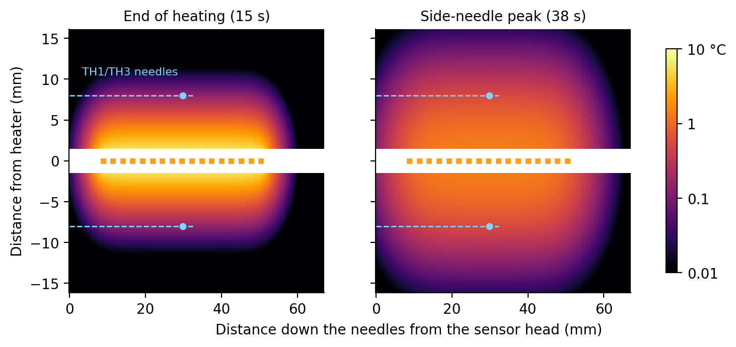
with the second term only after \(t_0\), \(P_i = 1.994/17 = 0.117\) W, and \(z_i = 8.8 + 2.6\,(i-1)\) mm the position of resistor \(i\) along the needle. TH1 and TH3 sit at \(z = 29.8\) mm, the middle of the heated section, and \(r = 8\) mm. TH2 sits on the heater needle, 3.68 mm past the last resistor. Figure 10 shows the resulting temperature field.
Figure 10. Soil temperature rise around the heater (logarithmic color scale, like the website's colormap), at the end of heating and at the side-needle peak. The orange marks are the 17 resistors (the heater needle itself is blank, because the model gives no value inside it); the dashed lines are the side needles, which end about 32 mm below the board. Heat leaks past both ends of the heater, which an infinite line would never do.
6.2 "Grid" resolution, time steps and boundary conditions in the twin
Many soil models divide the soil into a grid and step forward in time (finite differences or finite elements), and then grid spacing and time step control the accuracy. The twin has no grid. Both the line-source and the point-source solutions are exact formulas: the temperature at any point and time is computed directly, independently of every other point. So there is no numerical diffusion and no stability limit. What the twin does choose:
Item
Value
Why
Heater discretization
17 point sources, 2.6 mm apart
One per real resistor, at its real position
Stored temperature series
every 0.25 s
Smooth chart lines
Simulated readings
every 1 s, 64-reading averages, 14-bit codes
What the firmware would record
Website colormap
114 × 56 pixels over 67 × 32 mm (about 0.6 mm per pixel), refreshed every 0.25 s
For display only; each pixel is computed exactly
Special functions
erfc to 1.2 × 10⁻⁷; \(E_1\) by series and continued fraction
Errors far below a millikelvin
Boundary and initial conditions are those of Section 5.2, applied in three dimensions: uniform soil in every direction (no soil surface, no board or epoxy), uniform starting temperature, \(\Delta T \to 0\) far away, and zero-size needles that store no heat and touch the soil perfectly. The heater power is the PWM average; the 100 Hz flicker is not simulated (8 mm of soil smooths it out almost completely). TH4 on the board is held at the starting temperature because heat flow into the board is not modeled.
6.3 Why the twin's estimate differs from the soil values
The twin runs the measurement in two directions, like a real experiment:
Forward (the "truth"): the 17-point-source soil of Section 6.1, plus the electronics: 14-bit codes, averaging, one sample per second, subtracting the background.
Inverse (the "analysis"): what simple firmware would do: fit the ideal pulsed line source (Section 5.3) to TH1's rise, with the nominal 8 mm spacing.
Two analysis choices decide how close the answer comes. Take first a simple analysis that divides the power by the resistor-end-to-end length, 43.2 mm, and fits the whole 105 s record of a 90 s cooling phase. For the Hodgeman soil it reports \(\lambda = 1.331\) W m⁻¹ K⁻¹ (+3.7%) and \(C = 2.406\) MJ m⁻³ K⁻¹ (+2.6%). Three separate effects add up to that, and it is worth keeping them apart because they have different cures:
Effect
\(\lambda\)
\(C\)
Cure
1. Heated-length bookkeeping. Dividing the power by 43.2 mm (resistor end to resistor end) instead of the effective 44.2 mm (Section 5.5) makes \(q'\) 2.3% too high. Both properties scale with \(q'\).
+2.3%
+2.3%
Use 17 × 2.6 mm, or calibrate
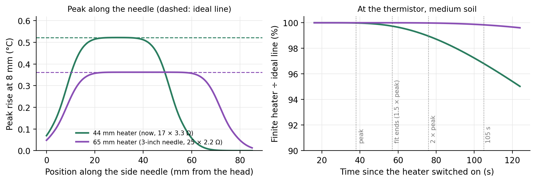
2. Finite heater (end effect). Heat also flows past the two ends of the heater. At the thermistor, midway along, the curve matches the ideal line through the peak, then falls below it late in the tail (Figure 11, right). Here the fit runs to 105 s. Late in the tail the ideal line depends on \(\lambda\) alone (\(\Delta T \approx Q'/(4\pi\lambda t)\)), so a lower tail pushes the fitted \(\lambda\) up; \(C\), set mainly by the peak height, barely moves, so \(\alpha = \lambda/C\) rises too.
+1.5%
+0.4%
Fit only to just past the peak (Section 7.6)
3. Quantization, sampling and background subtraction. One ADC step is 0.006 °C; the fit's RMS misfit is about 0.003 °C.
≈ −0.1%
≈ −0.1%
Small here. Without noise it can reach about ±0.8%, depending on where the baseline falls within one ADC step; real noise averages it out.
The effects multiply: \(1.023 \times 1.015 \times 0.999 \approx 1.037\) for \(\lambda\) and \(1.023 \times 1.004 \times 0.999 \approx 1.026\) for \(C\), the +3.7% and +2.6% above. The website uses the better choices: the effective length and a fit from heater-on to 1.5 times the measured peak time. It reports \(\lambda = 1.285\) (+0.1%), \(C = 2.344\) (−0.0%) and \(\alpha = 0.548\) mm² s⁻¹ for this soil, from 57 one-second readings (Sections 7.6–7.8).
Figure 11. Left: peak temperature rise along the side needle for the current 44 mm heater (green) and a 65 mm heater (purple), with the ideal line for each (dashed). Near the middle of the heater, where the thermistors sit, the finite heater reaches the ideal peak. Right: the finite heater's curve divided by the ideal line's at the thermistor (medium soil). The two agree to better than 0.1% at the peak (38 s) and to 0.3% where the fit ends, at 1.5 times the peak time (57 s); by twice the peak time (76 s) the gap is 1%, and by 105 s the finite heater is 3% lower. The longer heater stays within 0.4% throughout.
A real sensor adds more differences that the twin deliberately leaves out, because they need measurements to quantify: the needles' own radius and heat capacity, which shift and rescale the peak (earlier and higher, or later and lower, depending on whether the needles store less or more heat per volume than the soil; Knight et al. 2012); epoxy, contact resistance, and air gaps around the needles; the exact spacing after assembly and insertion; heater resistance changing slightly as it warms; and the soil not being uniform. That is why heat-pulse sensors are usually calibrated: measure a material with known properties (water stabilized with agar is common), and adjust the effective spacing until the sensor reads correctly. That absorbs a constant bias in \(C\), including the heated-length bookkeeping above, but not in \(\lambda\): in the line-source analysis \(\lambda\) does not depend on \(r\) at all. Getting \(\lambda\) right needs the correct \(q'\), or a second check against a material of known conductivity (water, about 0.6 W m⁻¹ K⁻¹).
And the "true" soil values are measurements too. The reference values come from a KD2 Pro SH-1, a commercial dual-needle probe with its own geometry, processing and uncertainty. Agreement within a few percent between two different instruments is good.
6.4 A real KD2 Pro curve
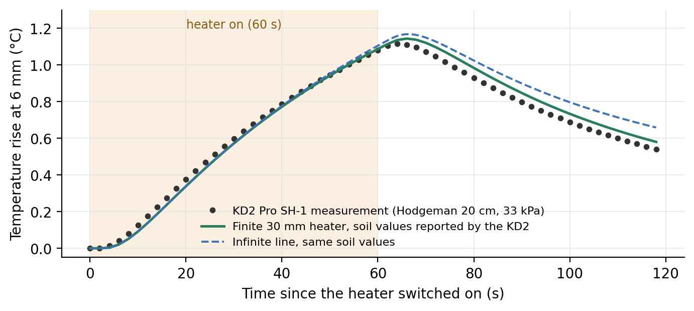
The Kansas dataset stores the raw temperature rise that the KD2 Pro recorded for each reading. The SH-1 probe has two 30 mm needles 6 mm apart and heated this core for 60 s at 18.3 W m⁻¹.
Figure 12. KD2 Pro SH-1 measurement for the twin's default soil (dots), a finite 30 mm heater with the soil values the KD2 reported (green), and an infinite line with the same values (dashed). Neither ideal model matches the measurement exactly: the data sit above both during heating and below both after the peak, though the finite heater comes closer.
Figure 12 shows the curve. One point first: the KD2 computed its reported \(\lambda\) and \(C\) from this same curve with its own analysis, which we do not know in detail. So any gap between those values and our fit is first a difference between two analyses of identical data. With that in mind, here is what the curve teaches, with numbers checked by simulation:
The finite length matters more with a long pulse on a short probe. Simulate the SH-1 geometry (30 mm heater, 6 mm spacing, 60 s at 18.3 W m⁻¹) in the reported soil and fit the ideal line to that noise-free, finite-heater curve over the same 118 s: the fit returns \(\lambda = 1.407\) (+9.7%) and \(C = 2.342\) (−0.1%). The heat-capacity estimate is almost untouched; the conductivity is not.
Finite length does not explain everything. Fitting the ideal line to the measured curve gives \(\lambda \approx 1.56\) and \(C \approx 2.27\). The finite length accounts for about half of the conductivity difference and none of the heat-capacity difference. The rest comes from things neither ideal model includes, such as the needles' own radius and heat capacity (Knight et al. 2012), contact between needle and soil, and the instrument's own processing; this one curve cannot separate them.
The peak comes only 4–6 s after the heater stops, and the readings are 2 s apart, so single-point peak methods are fragile here: moving \(t_m\) from 64 s to 62 or 66 s moves \(\alpha\) by +67% or −25%.
7. What if...? Design choices, one at a time
With the equations in hand we can ask design questions and answer them with numbers. Each question below changes one thing and keeps everything else as it is now.
7.1 How to read this section
The "truth" is the twin's finite-heater model (Section 6.1): 17 point sources (25 for the long-needle case) in uniform, ideal soil.
The "analysis" fits the ideal pulsed line source (Section 5.3) with \(q'\) = average power ÷ (number of resistors × 2.6 mm) and the nominal spacing, to one-second samples from heater-on to 1.5 times the peak time.
Record length: fitting to 1.5 times the peak time needs about 145 s of record after heater-on in the dry soil at 8 mm, and about 220 s at 10 mm (Table B, last column). That is why the default cooling phase is 150 s (Section 7.8).
No noise is added. The fitted values therefore show only the model error: what the ideal line misses about the real, finite heater. Real sensors add noise, spacing errors, needle heat capacity and contact effects (Section 6.3). The "ADC steps" column shows how big the signal is compared with the smallest step the electronics can resolve (about 0.0063 °C), which is a fair guide to how much noise will matter.
Three measured Kansas soils cover the range of diffusivities:
Soil
Kansas Mesonet core and state
\(\lambda\) (W m⁻¹ K⁻¹)
\(C\) (MJ m⁻³ K⁻¹)
\(\alpha\) (mm² s⁻¹)
Dry
Miami 5 cm, oven-dry
0.244
1.349
0.181
Medium
Hodgeman 20 cm, 33 kPa (the twin's default)
1.283
2.345
0.547
Wet sandy
Lake City 5 cm, sandy loam, saturated
2.159
1.944
1.111
The heater power is the same in every case (1.994 W average, 85% duty at 12 V), except the long-needle case, which needs different resistors (Section 7.5).
7.2 Two rules of thumb you can do on a calculator
From the short-pulse solution (Section 5.4), treating the pulse as if it were released all at once at its midpoint:
These are approximations. They work within a few percent while the pulse is short compared with \(r^2/(4\alpha)\), and fail for long pulses (Section 7.4). The comparisons below use the full pulsed line-source solution of Section 5.3, which is what the rules approximate. Check them on the present design (medium soil, \(r\) = 8 mm, \(t_0\) = 15 s, \(Q'\) = 677 J m⁻¹):
By hand. Only \(r\) changes. \(r^2/(4\alpha)\) becomes 16.5 s at 6 mm and 45.7 s at 10 mm, so \(t_m \approx\) 24.0 s and 53.2 s (full solution: 26.0 s and 54.0 s). At 6 mm the time rule is 8% low, because the 15 s pulse is nearly as long as \(r^2/(4\alpha)\). The peak scales with \(1/r^2\): \(677/(2.718\,\pi \times 0.006^2 \times 2.345\times10^6) = 0.939\) °C at 6 mm and 0.338 °C at 10 mm (full solution: 0.909 and 0.336 °C).
What changes.
Signal: 6 mm gives about 1.7 times today's peak, 10 mm about 0.64 times.
Sensitivity to spacing error: since \(C \propto 1/r^2\), a 0.1 mm error costs \(1-(r/(r+0.1))^2\): 3.3% at 6 mm, 2.5% at 8 mm, 2.0% at 10 mm. Closer needles need tighter spacing tolerance.
Model error: with the heater unchanged, a wider gap makes the heater "shorter" relative to the distance heat must travel, so the end effect grows: at 10 mm the fitted \(\lambda\) is +0.8% to +1.6% and \(C\) +0.4% to +0.6%; at 6 mm both stay within 0.1%.
Not in this model: the needles themselves (2.77 mm outside diameter for 12 gauge) take up a larger share of a 6 mm gap, so the effects of needle radius and heat capacity that the ideal model ignores (Knight et al. 2012) become more important as the gap shrinks. Our 12-gauge needles are already thicker than the roughly 1.3 mm needles of typical research probes, so those effects are likely larger here than in most published sensors.
7.4 What if we heat for 8, 15 or 60 seconds?
The Kansas readings in this chapter were taken with a KD2 Pro SH-1, which heats for 60 s (Section 6.4). Today's dual-probe sensors typically heat for 8–15 s; ours defaults to 15 s, and 60 s remains available only as a setting.
By hand. The power per meter stays 45.11 W m⁻¹, so the energy is \(Q' = 45.11 \times t_0\): 361, 677 and 2706 J m⁻¹. For 8 s: \(t_m \approx 29.2 + 4 = 33.2\) s and \(\Delta T_m \approx 361/1282 = 0.282\) °C (full solution: 33.6 s and 0.281 °C). For 60 s the rules give 59.2 s and 2.11 °C, but the full solution gives 74.3 s and 1.867 °C: the rules of thumb fail. The time rule even puts the peak before the heater switches off at 60 s. A 60 s pulse lasts longer than the 29 s the heat needs to reach the thermistor, so it no longer behaves like a single burst. Use the full equations of Section 5.4.
What changes.
Signal: grows with the energy, a little less than proportionally for long pulses: 8 s gives 44 ADC steps in the medium soil, 15 s gives 83, and 60 s (four times the energy of 15 s) gives 295, 3.6 times as many.
Heating of the soil next to the needle: the soil touching the heater needle warms much more than the soil at the thermistors. Beside a resistor (between resistors it is about 10% less, and the model ignores the needle wall, which would even this out): in the medium soil 5.2 °C (8 s), 6.8 °C (15 s) and 10.5 °C (60 s); in the dry soil 14.4, 21.3 and 39.5 °C. Strong local heating can push water away from the heater, which changes the very property being measured; this model does not include it, so large local rises are a warning sign, not a computed error.
Model error: small for 8 and 15 s. For 60 s it grows in high-diffusivity soil (+5.7% in \(\lambda\), −0.1% in \(C\) for the wet sandy soil), because by the time of the peak the heat has spread well past the ends of the heater.
Time and battery: the energy drawn from the battery is proportional to \(t_0\), and a longer pulse delays the peak and the end of the measurement.
7.5 What if the needles were 3 inches long?
A 3-inch (76 mm) needle has room for a 65 mm heater: 25 resistors at 2.6 mm, heater midpoint about 40 mm below the board (the side thermistors would move there too). The catch is the 12 V supply: 25 × 3.3 Ω = 82.5 Ω would cut the power to about 1.4 W. Keeping about 2 W needs about the same total resistance as now, so 25 × 2.2 Ω = 55 Ω. By Ohm's law (Section 2.2) that gives 2.03 W average, spread over 65 mm: \(q' = 31.27\) W m⁻¹, 31% less than now.
Signal: the peak falls from 0.522 to 0.362 °C in the medium soil (83 to 57 ADC steps). Heating 22 s instead of 15 s would restore it.
Model error: essentially zero in all three soils. But with the effective length and a fit to 1.5 times the peak time, today's 44 mm heater is already within +0.5% in \(\lambda\) and +0.1% in \(C\) (worst of the three soils), so the gain is about half a percent.
Bending: a needle held at one end bends in proportion to its free length cubed for a sideways force at the tip (to the fourth power for a force spread along it). The side needles, which set the spacing, now end about 32 mm below the board; moving the thermistors to the new heater midpoint would make them about 1.3–1.5 times longer, so they would bend roughly 2–4 times more for the same force during insertion. Because a 0.1 mm change in spacing already costs 2.5% in \(C\), this is likely to cost more accuracy than the longer heater gains.
7.6 What if we fit more, or less, of the curve?
This question matters more than the needle length. The peak's height and timing carry most of the information: the height mainly sets \(C\), the timing sets \(\alpha\). The tail is where the ideal line and the real sensor agree least. For the finite heater, the curve matches the ideal line through the peak and departs from it only late in the tail (Figure 11, right). The effects the model leaves out, such as the needles' own heat capacity, imperfect contact, heat left from a previous pulse and the soil's natural temperature drift, also show up mostly in the tail. So the further past the peak we fit, the more the fit is pulled by the part of the curve the ideal line gets wrong. This agrees with advice from G. J. Kluitenberg (personal communication, May 2026): fitting the tail, the part of least agreement, is a common mistake, and the fit should end just past the peak.
Without noise. Errors of the fitted \(\lambda\) / \(C\) for today's heater (8 mm, 15 s), by how far the fit runs:
Soil
Peak time
to 1.5 \(t_m\)
to 2 \(t_m\)
to 3 \(t_m\)
fixed 105 s
fixed 300 s
Dry
96.3 s
+0.1% / ±0.0%
+0.3% / +0.1%
+1.2% / +0.4%
±0.0% / ±0.0%
+1.4% / +0.4%
Medium
37.9 s
+0.2% / +0.1%
+0.6% / +0.2%
+1.8% / +0.4%
+1.5% / +0.4%
+7.9% / +1.0%
Wet sandy
24.2 s
+0.5% / +0.1%
+1.2% / +0.3%
+3.2% / +0.5%
+5.7% / +0.6%
+13.9% / +0.4%
With noise. The one argument for fitting further is that more points average out noise. To test it, we added independent random noise of 5 mK to each one-second reading (about one ADC step; the background is the mean of ten noisy readings), repeated each fit 200 times, and report the mean error ± the standard deviation of \(\lambda\):
Soil (peak time)
to 1.1 \(t_m\)
to 1.25 \(t_m\)
to 1.5 \(t_m\)
to 2 \(t_m\)
to 3 \(t_m\)
Dry (96 s)
0.0 ± 0.2%
0.0 ± 0.2%
0.1 ± 0.2%
0.4 ± 0.2%
0.4 ± 0.2%
Medium (38 s)
0.1 ± 0.7%
0.1 ± 0.5%
0.2 ± 0.4%
0.5 ± 0.4%
1.8 ± 0.4%
Wet sandy (24 s)
0.1 ± 1.0%
0.3 ± 0.7%
0.5 ± 0.5%
1.2 ± 0.4%
3.1 ± 0.4%
The error grows with the window, and the scatter shrinks only a little. Going from 2 to 3 times the peak time buys almost no precision but more than doubles the error in the medium and wet soils.
The best balance is about 1.25–1.5 times the peak time. Ending right at the peak (1.1 times) lets the scatter grow in wet soil, because the peak time itself becomes uncertain.
\(C\) hardly depends on the window (mean errors 0.0–0.5%, scatter ±0.1–0.4% in every case). The window matters for \(\lambda\) and \(\alpha\), which the tail drags upward.
The website and the planned firmware therefore fit from heater-on to 1.5 times the measured peak time. Readings recorded after that are kept, for plotting and quality checks, but not fitted. These tests assume independent noise and an ideal soil; the best window should be confirmed with bench data.
7.7 All cases in two tables
Table A. Signal. Peak rise at the thermistor and the maximum rise of the soil touching the heater needle (at its 1.385 mm outer radius, beside the middle resistor; point-source model, needle wall ignored).
Case
Soil
\(q'\) (W m⁻¹)
\(Q'\) (J m⁻¹)
Peak rise (°C)
ADC steps
Peak time (s)
Soil next to heater, max rise (°C)
Now: 44 mm heater, 8 mm, 15 s
Dry
45.1
677
0.916
145
96.3
21.3
Medium
45.1
677
0.522
83
37.9
6.8
Wet sandy
45.1
677
0.611
97
24.2
5.1
Spacing 6 mm
Dry
45.1
677
1.625
257
58.0
21.3
Medium
45.1
677
0.909
144
26.1
6.8
Wet sandy
45.1
677
1.019
161
19.2
5.1
Spacing 10 mm
Dry
45.1
677
0.586
93
144.8
21.3
Medium
45.1
677
0.336
53
53.6
6.8
Wet sandy
45.1
677
0.399
63
31.4
5.1
Heat 8 s
Dry
45.1
361
0.489
77
92.5
14.4
Medium
45.1
361
0.281
44
33.6
5.2
Wet sandy
45.1
361
0.335
53
19.1
4.1
Heat 60 s
Dry
45.1
2706
3.604
571
124.8
39.5
Medium
45.1
2706
1.861
295
74.1
10.5
Wet sandy
45.1
2706
1.840
291
65.0
7.4
3-inch needle, 65 mm heater
Dry
31.3
469
0.635
101
96.4
14.8
Medium
31.3
469
0.362
57
38.0
4.7
Wet sandy
31.3
469
0.424
67
24.3
3.6
Table B. What the analysis reports (fitted value, with the error relative to the true soil value in parentheses; fit from heater-on to 1.5 times the peak time).
Case
Soil
\(\lambda\) fitted (W m⁻¹ K⁻¹)
\(C\) fitted (MJ m⁻³ K⁻¹)
\(\alpha\) fitted (mm² s⁻¹)
Record fitted (s)
Now: 44 mm heater, 8 mm, 15 s
Dry
0.244 (+0.1%)
1.350 (±0.0%)
0.181 (+0.1%)
144
Medium
1.285 (+0.2%)
2.346 (+0.1%)
0.548 (+0.1%)
56
Wet sandy
2.169 (+0.5%)
1.947 (+0.1%)
1.114 (+0.3%)
36
Spacing 6 mm
Dry
0.244 (±0.0%)
1.349 (±0.0%)
0.181 (±0.0%)
86
Medium
1.283 (±0.0%)
2.345 (±0.0%)
0.547 (±0.0%)
39
Wet sandy
2.161 (+0.1%)
1.944 (±0.0%)
1.112 (+0.1%)
28
Spacing 10 mm
Dry
0.246 (+0.8%)
1.354 (+0.4%)
0.182 (+0.4%)
217
Medium
1.296 (+1.0%)
2.355 (+0.4%)
0.550 (+0.6%)
80
Wet sandy
2.193 (+1.6%)
1.956 (+0.6%)
1.121 (+1.0%)
47
Heat 8 s
Dry
0.244 (+0.1%)
1.349 (±0.0%)
0.181 (±0.0%)
138
Medium
1.284 (+0.1%)
2.346 (±0.0%)
0.547 (+0.1%)
50
Wet sandy
2.163 (+0.2%)
1.945 (+0.1%)
1.112 (+0.1%)
28
Heat 60 s
Dry
0.245 (+0.2%)
1.350 (+0.1%)
0.181 (+0.1%)
187
Medium
1.304 (+1.6%)
2.352 (+0.3%)
0.554 (+1.3%)
111
Wet sandy
2.282 (+5.7%)
1.943 (−0.1%)
1.174 (+5.7%)
97
3-inch needle, 65 mm heater
Dry
0.244 (±0.0%)
1.349 (±0.0%)
0.181 (±0.0%)
144
Medium
1.283 (±0.0%)
2.345 (±0.0%)
0.547 (±0.0%)
56
Wet sandy
2.159 (±0.0%)
1.944 (±0.0%)
1.111 (±0.0%)
36
What the tables say.
With the effective heated length and a fit to 1.5 times the peak time, the present design's finite-length model error is 0.5% or less in \(\lambda\) and 0.1% or less in \(C\) across dry to wet sandy soil. Needle size, contact and noise come on top of this.
Needle spacing is the biggest practical lever: every 0.1 mm of spacing error costs about 2.5% in \(C\), more than any model error above. Measuring or calibrating each sensor's effective spacing matters more than lengthening the needles.
Longer needles remove the remaining model error but reduce the signal by about 30% and bend more.
Longer pulses buy signal at the cost of strong heating next to the needle; 15 s is a reasonable middle.
7.8 Choosing settings: defaults and when to change them
Every setting below can be changed on the website and, in the planned firmware, on the sensor itself. The defaults are chosen to work reasonably in most soils with the present needles (8 mm spacing, 44 mm heater); change them when you know in advance what conditions you will measure.
Setting
Default
Why
Background
10 s
Ten one-second readings to average for the starting temperature.
Heating
15 s at 85% duty (about 2.0 W, 677 J m⁻¹)
A peak of 0.41–1.05 °C (5th to 95th percentile of the 1,448 Kansas soil states), or about 65–165 ADC steps, while the soil touching the needle warms by 5–18 °C.
Cooling
150 s (165 s of record after heater-on)
The median peak comes 39 s after heater-on and the latest, in an oven-dry core, at 98 s. The record covers 1.5 times the peak time in every state, with room to spare for locating the peak.
Analysis
\(q'\) over 44.2 mm; fit from heater-on to 1.5 times the measured peak time
Finite-length model error 0.3% or less for \(\lambda\) and 0.1% or less for \(C\) (5th to 95th percentile of the Kansas states). The website warns if the record ends before the peak.
Why can the peak come 96 s after a 15 s pulse? The heating time only shifts the peak by about half the pulse (Section 7.2). The peak time is set mainly by \(r^2/(4\alpha)\): how long heat needs to cross the gap. Oven-dried soil has the lowest diffusivity in the Kansas data (\(\alpha \approx 0.18\) mm² s⁻¹, because air-filled pores conduct heat poorly), so heat needs \(0.008^2/(4 \times 0.18\times10^{-6}) \approx 88\) s to cross 8 mm, and the peak arrives near 96 s. Oven-dried cores are the extreme; field soils are rarely that dry, and most peaks come within 30–65 s.
When to change them (numbers from the same ideal model; confirm on the bench):
Wet or sandy soils (high diffusivity). The peak comes early (about 20–25 s), so a shorter cooling phase (60–90 s) is enough. Wet soils give the smallest peaks, so a longer pulse helps the signal; in the wet sandy soil 20 s gives a 0.79 °C peak with +0.8% in \(\lambda\), and 30 s gives 1.12 °C with +1.7% (Section 7.4). Averaging repeated measurements is the other way to beat noise.
Dry soils (low diffusivity). The peak comes late (90–100 s in oven-dry soil), so keep the 150 s cooling phase. The signal is large, but the soil next to the heater gets hot: about 21 °C at 15 s in the oven-dry example. Lowering the duty to 50% keeps a 0.54 °C peak and brings that down to about 12.5 °C; do not lengthen the pulse.
How often to measure. Each pulse leaves heat behind that fades slowly, and the analysis subtracts a flat background. If the next measurement starts while the needles are still cooling, the falling background biases the result. Assuming identical pulses and no natural temperature drift, the added error in \(\lambda\) / \(C\) is:
Interval
Dry
Medium
Wet sandy
5 min
+19% / +17%
+4.0% / +3.6%
+1.8% / +1.4%
15 min
+3.3% / +2.7%
+0.6% / +0.4%
+0.6% / +0.2%
30 min
+0.9% / +0.7%
+0.3% / +0.1%
+0.5% / +0.2%
60 min
+0.3% / +0.2%
+0.2% / +0.1%
+0.5% / +0.1%
no previous pulse
+0.1% / ±0.0%
+0.2% / +0.1%
+0.5% / +0.1%
Every 15 minutes is fine in moist soil; dry soil needs about 30 minutes, and hourly measurements are clean in every soil. Fitting a sloped background, rather than a flat one, would reduce this error and also handle the soil's natural daily temperature swing.
Very dry soil or wider needles. If the website reports that the record ended before the peak, lengthen the cooling phase.
8. The whole chain in one table
For the Hodgeman soil (true values \(\alpha = 0.547\) mm² s⁻¹, \(\lambda = 1.283\), \(C = 2.345\)), as the website computes it: effective heated length, 14-bit readings once per second, fit to 1.5 times the peak time.
#
Quantity
How we get it
Example
1
Heater current
Ohm's law around the loop
0.2045 A
2
Heater power, average
\(I^2R\) × duty
1.994 W
3
Power per meter \(q'\)
power ÷ 44.2 mm (17 × 2.6 mm)
45.11 W m⁻¹
4
Thermistor code
divider + 14-bit ADC, VREF cancels
8663 at 22 °C
5
Thermistor resistance
\(R_\text{ref}\,\text{code}/(16384-\text{code})\)
11.22 kΩ
6
Temperature
beta equation
22.00 °C
7
Rise at the side needle
temperature − background average
peak ≈ 0.52 °C at 38 s
8
\(\alpha\), \(\lambda\), \(C\)
fit the pulsed line source up to 1.5 times the peak time
0.548 mm² s⁻¹, 1.285, 2.344
9
Water content
de Vries: \((C - \rho_b c_s)/C_w\)
≈ 0.32 m³ m⁻³
9. Glossary
ADC
Analog-to-digital converter: turns a voltage into a whole number (code).
AREF / VREF
The ADC's reference voltage (its ruler). Here both are the same node, which makes the measurement ratiometric.
Capacitor
A part that stores charge; smooths voltages and, with a resistor, sets a time constant.
Duty cycle
Fraction of time a switch is on during PWM.
GND
Ground, the 0 V reference point.
MOSFET
An electronic switch (Q1) that a processor pin can open and close.
NTC thermistor
Resistor whose resistance falls as temperature rises.
PWM
Pulse-width modulation: fast on/off switching to set an average power.
Ratiometric
A measurement taken as a ratio, so a common supply voltage cancels.
Self-heating
A sensor warmed by the very current used to read it.
Superposition
Adding solutions of a linear equation; used to switch the heater off.
Time constant \(\tau\)
\(R \times C\): time to reach 63% of a step change.
Blackwell, J. H. (1954). A transient-flow method for determination of thermal constants of insulating materials in bulk. Part I—Theory. Journal of Applied Physics, 25, 137–144. doi:10.1063/1.1721592
Bristow, K. L., Bilskie, J. R., Kluitenberg, G. J., & Horton, R. (1995). Comparison of techniques for extracting soil thermal properties from dual-probe heat-pulse data. Soil Science, 160, 1–7. doi:10.1097/00010694-199507000-00001
Bristow, K. L., Kluitenberg, G. J., & Horton, R. (1994). Measurement of soil thermal properties with a dual-probe heat-pulse technique. Soil Science Society of America Journal, 58, 1288–1294. doi:10.2136/sssaj1994.03615995005800050002x
Campbell, G. S., Calissendorff, C., & Williams, J. H. (1991). Probe for measuring soil specific heat using a heat-pulse method. Soil Science Society of America Journal, 55, 291–293. doi:10.2136/sssaj1991.03615995005500010052x
Carslaw, H. S., & Jaeger, J. C. (1959). Conduction of heat in solids (2nd ed.). Oxford University Press.
de Vries, D. A. (1963). Thermal properties of soils. In W. R. van Wijk (Ed.), Physics of plant environment (pp. 210–235). North-Holland.
Kluitenberg, G. J., Bristow, K. L., & Das, B. S. (1995). Error analysis of heat pulse method for measuring soil heat capacity, diffusivity, and conductivity. Soil Science Society of America Journal, 59, 719–726. doi:10.2136/sssaj1995.03615995005900030013x
Kluitenberg, G. J., Ham, J. M., & Bristow, K. L. (1993). Error analysis of the heat pulse method for measuring soil volumetric heat capacity. Soil Science Society of America Journal, 57, 1444–1451. doi:10.2136/sssaj1993.03615995005700060008x
Knight, J. H., & Kluitenberg, G. J. (2004). Simplified computational approach for dual-probe heat-pulse method. Soil Science Society of America Journal, 68, 447–449. doi:10.2136/sssaj2004.4470
Knight, J. H., Kluitenberg, G. J., Kamai, T., & Hopmans, J. W. (2012). Semianalytical solution for dual-probe heat-pulse applications that accounts for probe radius and heat capacity. Vadose Zone Journal, 11(2). doi:10.2136/vzj2011.0112
Parker, N., Kluitenberg, G. J., Redmond, C., & Patrignani, A. (2022). A database of soil physical properties for the Kansas Mesonet. Soil Science Society of America Journal, 86, 1495–1508. doi:10.1002/saj2.20465
Numbers in this chapter come from the HP-SDI12-NANO design files and the digital twin (docs/sensor-model.js, docs/engine.js) as of September 29, 2026. Self-heating depends on how the thermistor is potted and is an estimate, not a measurement.
Appendix A. Parts list (HP-SDI12-NANO)
68 fitted parts in 25 lines, all on the top face (release BOM flat-nano/fab/HP-SDI12-NANO_BOM.csv, which also gives LCSC numbers). † No substitutes: sets accuracy or heater rating. J1 (cable) and J2 (programming clip) are bare plated holes, not parts.